Page Summary
-
This tutorial, although outdated and not recommended for Landsat Collection 2 data, provides methods for harmonizing Landsat ETM+ and OLI surface reflectance data using spectral transformation functions and techniques to create analysis-ready data and visualize time series.
-
The harmonization process involves applying a linear transformation to ETM+ data based on coefficients derived from OLS regression and standardizing band names between OLI and ETM+ sensors.
-
Functions are provided for cloud and shadow masking using the
pixel_qaband and for calculating spectral indices like Normalized Burn Ratio (NBR). -
The tutorial demonstrates how to create and visualize a 35+ year time series of Landsat data for a specific area of interest, showing how to filter collections, merge data from different sensors, and generate charts of spectral response over time.
-
Alternative transformation functions and additional context about the Dollar Lake fire, which is used as an example in the time series analysis, are also mentioned.
WARNING: The procedures described in this tutorial to harmonize Landsat ETM+ and OLI data are outdated and not recommended or necessary when working with Landsat Collection 2 surface reflectance data. For more information, see the FAQ entry on Landsat harmonization. Collection 1 data are deprecated and the code in this tutorial will no longer work or be updated.
This tutorial concerns harmonizing Landsat ETM+ surface reflectance to Landsat OLI surface reflectance. It provides:
- A spectral transformation function
- Functions to create analysis-ready data
- A time series visualization example
It is intended to be an end-to-end guide for harmonizing and visualizing a 35+ year regional time series of Landsat data that can be immediately applied to your own region(s) of interest.
Note that the coefficients for transforming ETM+ to OLI applies to TM as well. As such, within this tutorial, reference to ETM+ is synonymous with TM.
About Landsat
Landsat is a satellite imaging program that has been collecting moderate resolution Earth imagery since 1972. As the longest space-based Earth observation program, it provides a valuable temporal record for identifying spatiotemporal trends in landscape change. Thematic Mapper (TM), Enhanced Thematic Mapper Plus (ETM+), and Operational Land Imager (OLI) instrument data are used in this tutorial. They are closely related and relatively easy to consolidate into a consistent time series that produces a continuous record from 1984 to the present, at a cadence of 16 days per sensor with 30 meter spatial resolution. The Multispectral Scanner instrument extends the Landsat record back to 1972, but is not used in this tutorial. Its data are quite different, making integration with later sensors challenging. See Savage et al. (2018) and Vogeler et al. (2018) for examples of harmonization across all sensors.
Why harmonization
Roy et al. (2016) demonstrate that there are small, but potentially significant differences between the spectral characteristics of Landsat ETM+ and OLI, depending on application. Reasons you might want to harmonize datasets include: producing a long time series that spans Landsat TM, ETM+, and OLI, generating near-date intra-annual composites to reduce the effects of missing observations from ETM+ SLC-off gaps and cloud/shadow masking, or increase the observation frequency within a time series. Please see the linked manuscript above for more information.
Instructions
Functions
The following are a series of functions that are needed to harmonize ETM+ to OLI and generate analysis-ready data that will be used in the application section of this tutorial to visualize the spectral-temporal history of a pixel.
Harmonization
Harmonization is achieved via linear transformation of ETM+ spectral space to
OLI spectral space according to coefficients presented in
Roy et al. (2016) Table 2 OLS regression coefficients.
Band-respective coefficients are defined in the following dictionary with slope
(slopes) and intercept (itcps) image constants. Note that the y-intercept
values are multiplied by 10,000 to match the scaling of USGS Landsat surface
reflectance data.
var coefficients = {
  itcps: ee.Image.constant([0.0003, 0.0088, 0.0061, 0.0412, 0.0254, 0.0172])
             .multiply(10000),
  slopes: ee.Image.constant([0.8474, 0.8483, 0.9047, 0.8462, 0.8937, 0.9071])
};
ETM+ and OLI band names for the same spectral response window are not equal and
need to be standardized. The following functions select only reflectance bands
and the pixel_qa band from each dataset, and renames them according to the
wavelength range they represent.
// Function to get and rename bands of interest from OLI.
function renameOli(img) {
  return img.select(
      ['B2', 'B3', 'B4', 'B5', 'B6', 'B7', 'pixel_qa'],
      ['Blue', 'Green', 'Red', 'NIR', 'SWIR1', 'SWIR2', 'pixel_qa']);
}

// Function to get and rename bands of interest from ETM+.
function renameEtm(img) {
  return img.select(
      ['B1', 'B2', 'B3', 'B4', 'B5', 'B7', 'pixel_qa'],
      ['Blue', 'Green', 'Red', 'NIR', 'SWIR1', 'SWIR2', 'pixel_qa']);
}
Finally, define the transformation function, which applies the linear model to
ETM+ data, casts data type as Int16 for consistency with OLI, and reattaches
the pixel_qa band for later use in cloud and shadow masking.
function etmToOli(img) {
  return img.select(['Blue', 'Green', 'Red', 'NIR', 'SWIR1', 'SWIR2'])
      .multiply(coefficients.slopes)
      .add(coefficients.itcps)
      .round()
      .toShort()
      .addBands(img.select('pixel_qa'));
}
Cloud and shadow masking
Analysis ready data should have clouds and cloud shadows masked out. The
following function uses the CFmask (Zhu et al., 2015)
pixel_qa band included with each Landsat USGS surface reflectance image to set
pixels identified as cloud and cloud shadow to null.
function fmask(img) {
  var cloudShadowBitMask = 1 << 3;
  var cloudsBitMask = 1 << 5;
  var qa = img.select('pixel_qa');
  var mask = qa.bitwiseAnd(cloudShadowBitMask)
                 .eq(0)
                 .and(qa.bitwiseAnd(cloudsBitMask).eq(0));
  return img.updateMask(mask);
}
Spectral index calculation
The forthcoming application uses the normalized burn ratio (NBR) spectral index to represent the spectral history of a forested pixel affected by wildfire. NBR is used because Cohen et al. (2018) found that among 13 spectral indices/bands, NBR had the greatest signal to noise ratio with regard to forest disturbance (signal) throughout the US. It is calculated by the following function.
function calcNbr(img) {
  return img.normalizedDifference(['NIR', 'SWIR2']).rename('NBR');
}
In your own application, you may choose to use a different spectral index. Here is the place to alter or add an additional index.
Combine functions
Define a wrapper function for each dataset that consolidates all above functions for convenience in applying them to their respective image collections.
// Define function to prepare OLI images.
function prepOli(img) {
  var orig = img;
  img = renameOli(img);
  img = fmask(img);
  img = calcNbr(img);
  return ee.Image(img.copyProperties(orig, orig.propertyNames()));
}

// Define function to prepare ETM+ images.
function prepEtm(img) {
  var orig = img;
  img = renameEtm(img);
  img = fmask(img);
  img = etmToOli(img);
  img = calcNbr(img);
  return ee.Image(img.copyProperties(orig, orig.propertyNames()));
}
In your application, you might decide to include or exclude functions. Alter these functions as needed.
Time series example
The prepOli and prepEtm wrapper functions above can be mapped over Landsat
surface reflectance collections to create cross-sensor analysis-ready data to
visualize the spectral chronology of a pixel or region of pixels. In this
example, you will create a 35+ year time series and display the spectral history
for a single pixel. This particular pixel relates the recent history of a mature
Pacific Northwest conifer forest patch (Figure 1) that experienced some
perturbation in the 1980's and 90's and a high magnitude burn in 2011.
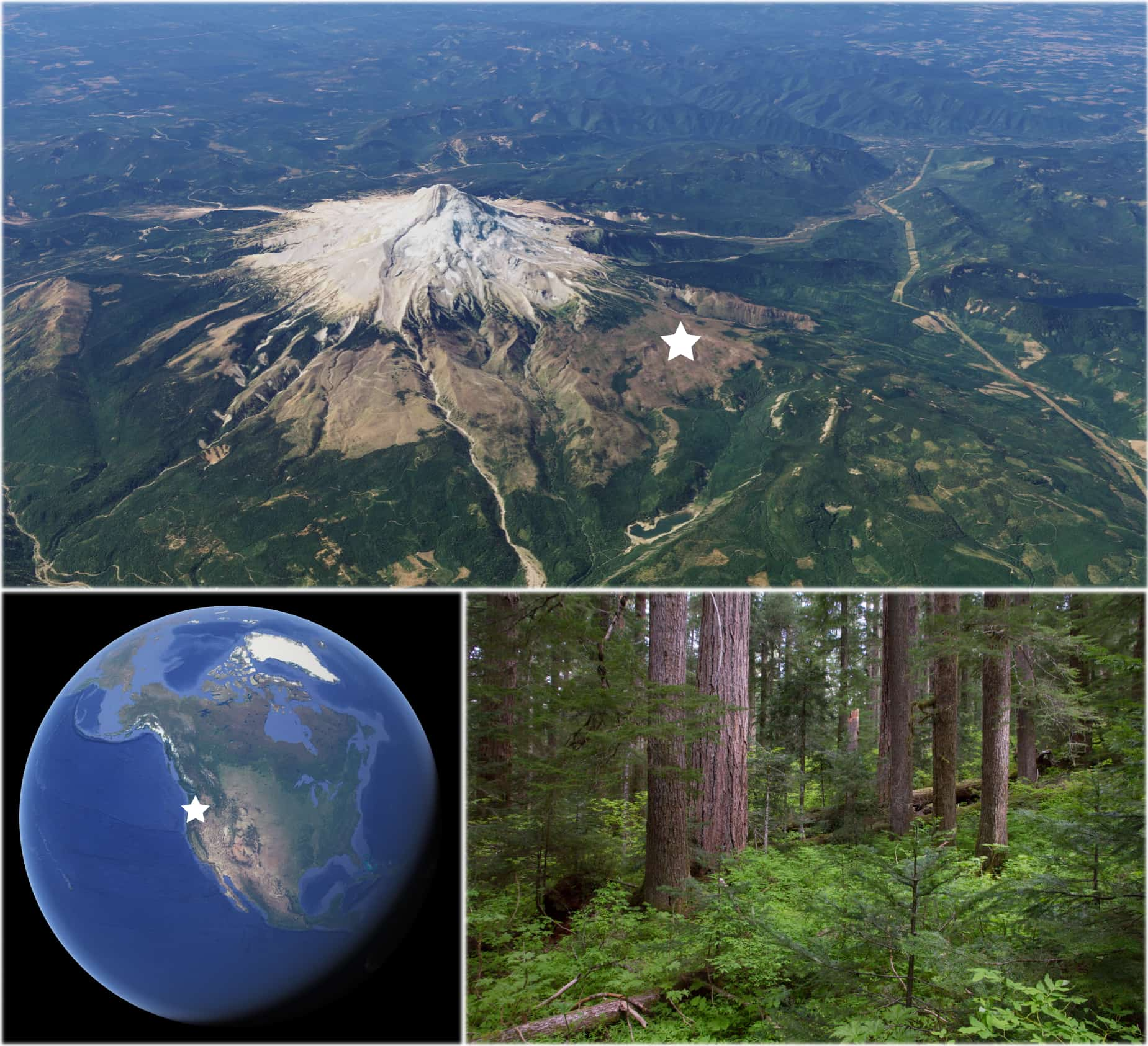
Figure 1. Location and site character for example area of interest. Mature Pacific Northwest conifer forest on the north slope of Mt Hood, OR, USA. Images courtesy of: Google Earth, USDA Forest Service, Landsat, and Copernicus.
Define an area of interest (AOI)
The result of this application is a time series of Landsat observations for a
pixel. An ee.Geometry.Point object is used to define the pixel's location.
var aoi = ee.Geometry.Point([-121.70938, 45.43185]);
In your application, you might select a different pixel. Do so by replacing the
above longitude and latitude coordinates. Alternatively, you can summarize
the spectral history of a group of pixels using other ee.Geometry object
definitions, such as ee.Geometry.Polygon() and ee.Geometry.Rectangle().
Please see the
Geometries
section of the Developer Guide for more information.
Retrieve Landsat sensor collections
Get Landsat USGS surface reflectance collections for OLI, ETM+, and TM.
Visit the links to learn more about each dataset.
var oliCol = ee.ImageCollection('LANDSAT/LC08/C01/T1_SR');
var etmCol = ee.ImageCollection('LANDSAT/LE07/C01/T1_SR');
var tmCol = ee.ImageCollection('LANDSAT/LT05/C01/T1_SR');
Define an image collection filter
Define a filter to constrain the image collections by the spatial boundary of the area of interest, peak photosynthesis season, and quality.
var colFilter = ee.Filter.and(
    ee.Filter.bounds(aoi), ee.Filter.calendarRange(182, 244, 'day_of_year'),
    ee.Filter.lt('CLOUD_COVER', 50), ee.Filter.lt('GEOMETRIC_RMSE_MODEL', 10),
    ee.Filter.or(
        ee.Filter.eq('IMAGE_QUALITY', 9),
        ee.Filter.eq('IMAGE_QUALITY_OLI', 9)));
Alter these filtering criteria as you wish. Identify other properties to filter by under the "Images Properties" tab of the data description pages linked above.
Prepare the collections
Merge the collections, apply the filter, and map the prepImg function over all
images. The result of the following snippet is a single ee.ImageCollection
that contains images from OLI, ETM+, and TM sensor collections that meet the
filter criteria, and are processed to analysis-ready NBR.
// Filter collections and prepare them for merging.
oliCol = oliCol.filter(colFilter).map(prepOli);
etmCol = etmCol.filter(colFilter).map(prepEtm);
tmCol = tmCol.filter(colFilter).map(prepEtm);

// Merge the collections.
var col = oliCol.merge(etmCol).merge(tmCol);
Make a times series chart displaying all observations
Inter-sensor harmony can be assessed qualitatively by plotting all observations
as a scatter plot where sensor is discerned by color. Earth Engine's
ui.Chart.feature.groups function provides this utility, but first the observed
NBR value must be added to each image as a property. Map a region reduce
function over the image collection that calculates the median of all pixels
intersecting the AOI and sets the result as an image property.
var allObs = col.map(function(img) {
  var obs = img.reduceRegion(
      {geometry: aoi, reducer: ee.Reducer.median(), scale: 30});
  return img.set('NBR', obs.get('NBR'));
});
In your own application, if your AOI is a large area, you might consider
increasing the scale and specifying bestEffort, maxPixels, tileScale
arguments for the reduceRegion function to ensure that the operation does not
exceed max pixels, memory, or timeout limitations. You can also replace the
median reducer with your preferred statistic. See the
Statistics of an Image Region
section of the Developer Guide for more information.
The collection can now be accepted by the ui.Chart.feature.groups function.
The function expects a collection and the names of collection object properties
to map to the chart. Here, the 'system:time_start' property serves as the
x-axis variable and 'NBR' as the y-axis variable. Note that the NBR property was
named by the reduceRegion function above based on the band name in the image
being reduced. If you use a different band (not 'NBR'), change the y-axis
property name argument accordingly. Finally, set the grouping (series) variable
to 'SATELLITE', to which distinct colors are assigned.
var chartAllObs =
    ui.Chart.feature.groups(allObs, 'system:time_start', 'NBR', 'SATELLITE')
        .setChartType('ScatterChart')
        .setSeriesNames(['TM', 'ETM+', 'OLI'])
        .setOptions({
          title: 'All Observations',
          colors: ['f8766d', '00ba38', '619cff'],
          hAxis: {title: 'Date'},
          vAxis: {title: 'NBR'},
          pointSize: 6,
          dataOpacity: 0.5
        });
print(chartAllObs);
A chart similar to Figure 2 will appear in the console after some processing time. Note several things:
- There are multiple observations per year.
- The time series is composed of three different sensors.
- There are no disernableable sensor-biases.
- Observation frequency varies annually.
- There is some intra-annual variance, which is consistent across years and relatively tight. Trying this with NDVI (img.normalizedDifference(['SWIR1', 'NIR']).rename('NDVI');) shows much greater intra- and inter-annual response variability.
- NBR remains high for the majority of the time series with some minor perturbations.
- A great, rapid reduction in NBR response results from a forest fire evident in
- Note however, that the fire (Dollar Lake) occurred in September of 2011. The error in detection year is due to the annual composite date range being July through August; changes occurring after this period are not picked until the next available non-null observation, which could be the next year or later.
- Vegetation recovery (increasing NBR response) begins two years after the major NBR loss is detected.
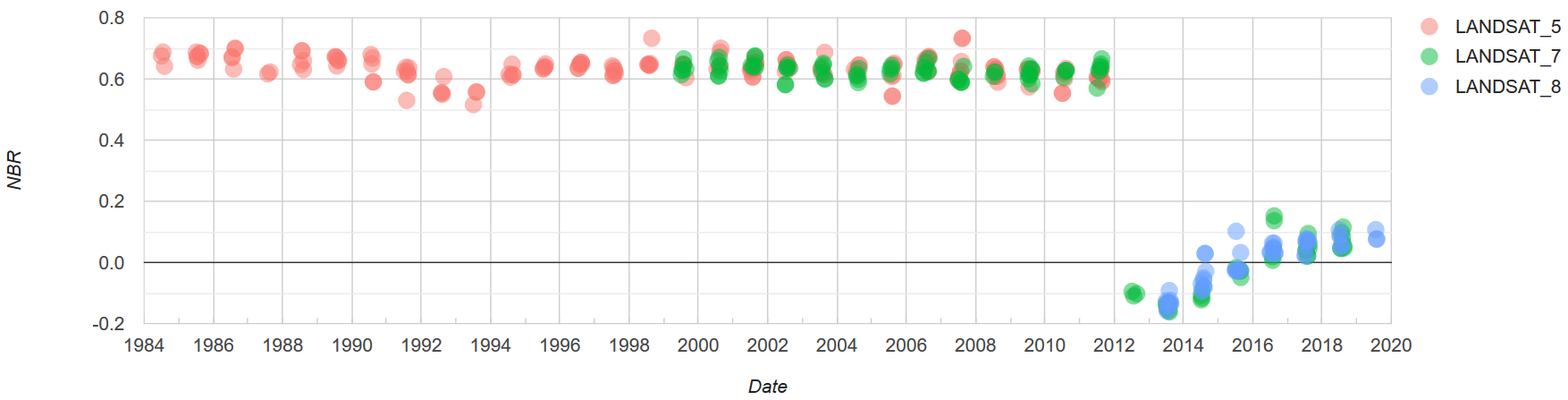
Figure 2. Spectral response time series chart for a single pixel with representation from Landsat TM, ETM+, and OLI. TM and ETM+ images are harmonized to OLI by linear transformation. Images are from July through August and are filtered for high quality.
Make a times series chart displaying annual median
To simplify and remove noise from the time series, intra-annual observation reduction can be applied. Here, median is used.
The first step is to group images by year. Add a new 'year' property to each
image by mapping over the collection setting 'year' from each image's
ee.Image.Date.
var col = col.map(function(img) {
  return img.set('year', img.date().get('year'));
});
The new 'year' property can be used to group images from the same year by a join. The join between a distinct image year collection and the complete collection provides same-year lists, from which median reductions can be performed. Subset the complete collection to a set of distinct year representatives.
var distinctYearCol = col.distinct('year');
Define a filter and a join that will identify matching years between the
distinct year collection (distinctYearCol) and the complete collection
(col). Matches will be saved to a property called 'year_matches'.
var filter = ee.Filter.equals({leftField: 'year', rightField: 'year'});
var join = ee.Join.saveAll('year_matches');
Apply the join and convert the resulting FeatureCollection to an ImageCollection.
var joinCol = ee.ImageCollection(join.apply(distinctYearCol, col, filter));

// Apply median reduction among matching year collections.
var medianComp = joinCol.map(function(img) {
  var yearCol = ee.ImageCollection.fromImages(img.get('year_matches'));
  return yearCol.reduce(ee.Reducer.median())
      .set('system:time_start', img.date().update({month: 8, day: 1}));
});
Change the ee.Reducer above if you prefer a statistic other than median to
represent the collection of images in a given year.
Finally, create a chart that displays the median NBR values from sets of inta-annual summer observations. Change the region reduction statistic as you like.
var chartMedianComp = ui.Chart.image
                          .series({
                            imageCollection: medianComp,
                            region: aoi,
                            reducer: ee.Reducer.median(),
                            scale: 30,
                            xProperty: 'system:time_start',
                          })
                          .setSeriesNames(['NBR Median'])
                          .setOptions({
                            title: 'Intra-annual Median',
                            colors: ['619cff'],
                            hAxis: {title: 'Date'},
                            vAxis: {title: 'NBR'},
                            lineWidth: 6
                          });
print(chartMedianComp);
A chart similar to Figure 3 will appear in the console after some processing time.
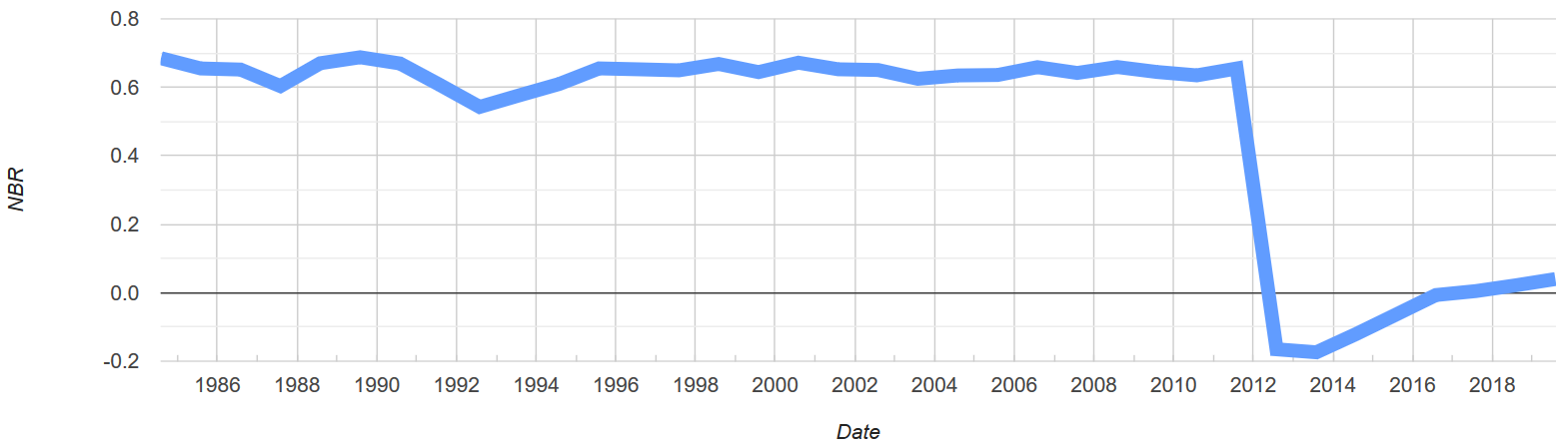
Figure 3. Median summer spectral response time series chart for a single pixel with representation from Landsat TM, ETM+, and OLI. TM and ETM+ images are harmonized to OLI by a linear transformation. Images are from July through August and are filtered for high quality.
Additional information
Alternative transformation functions
Roy et al. (2016) Table 2 provides OLS and RMA regression coefficients to transform ETM+ surface reflectance to OLI surface reflectance and vice versa. The above tutorial demonstrates only ETM+ to OLI transformation by OLS regression. Functions for all translation options can be found in the Code Editor script or the GitHub source script.
The Dollar Lake fire
The fire mentioned in this tutorial is the Dollar Lake fire, which occurred mid-September, 2011 on the northern slopes of Mt Hood, OR, USA. Visit this blog post and see Varner et al. (2015) for more information about it.