Page Summary
-
ImageCollectionvisualization can be displayed as an animation or a filmstrip of thumbnails. -
Preparation methods like filtering, compositing, and sorting are crucial for effective
ImageCollectionvisualization. -
Image visualization transforms numerical data into colors using parameters like bands, min/max values, and palettes.
-
The
getVideoThumbURL()function generates an animation from anImageCollection. -
The
getFilmstripThumbUrl()function creates a single static image from anImageCollection, concatenating images into a north-south series.
Images composing an ImageCollection can be visualized as either an
animation or a series of thumbnails referred to as a “filmstrip”. These
methods provide a quick assessment of the contents of an ImageCollection
and an effective medium for witnessing spatiotemporal change (Figure 1).
getVideoThumbURL()produces an animated image seriesgetFilmstripThumbURL()produces a thumbnail image series
The following sections describe how to prepare an ImageCollection for
visualization, provide example code for each collection visualization method,
and cover several advanced animation techniques.
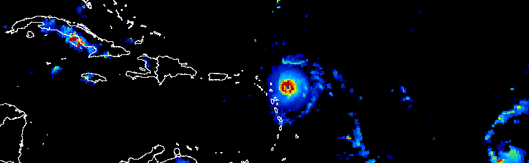
Figure 1. Animation showing a three-day progression of Atlantic hurricanes in
September, 2017.
Collection preparation
Filter, composite, sort, and style images within a collection to display only
those of interest or emphasize a phenomenon. Any ImageCollection can be
provided as input to the visualization functions, but a curated collection
with consideration of inter- and intra-annual date ranges, observation
interval, regional extent, quality and representation can achieve better
results.
Filtering
Filter an image collection to include only relevant data that supports the purpose of the visualization. Consider dates, spatial extent, quality, and other properties specific to a given dataset.
For instance, filter a Sentinel-2 surface reflectance collection by:
a single date range,
Code Editor (JavaScript)
var s2col = ee.ImageCollection('COPERNICUS/S2_SR')
  .filterDate('2018-01-01', '2019-01-01');
a serial day-of-year range,
Code Editor (JavaScript)
var s2col = ee.ImageCollection('COPERNICUS/S2_SR')
  .filter(ee.Filter.calendarRange(171, 242, 'day_of_year'));
a region of interest,
Code Editor (JavaScript)
var s2col = ee.ImageCollection('COPERNICUS/S2_SR')
  .filterBounds(ee.Geometry.Point(-122.1, 37.2));
or an image property.
Code Editor (JavaScript)
var s2col = ee.ImageCollection('COPERNICUS/S2_SR')
  .filter(ee.Filter.lt('CLOUDY_PIXEL_PERCENTAGE', 50));
Chain multiple filters.
Code Editor (JavaScript)
var s2col = ee.ImageCollection('COPERNICUS/S2_SR')
  .filterDate('2018-01-01', '2019-01-01')
  .filterBounds(ee.Geometry.Point(-122.1, 37.2))
  .filter('CLOUDY_PIXEL_PERCENTAGE < 50');
Compositing
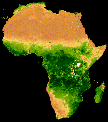
Composite intra- and inter-annual date ranges to reduce the number of images in a collection and improve quality. For example, suppose you were to create a visualization of annual NDVI for Africa. One option is to simply filter a MODIS 16-day NDVI collection to include all 2018 observations.
Code Editor (JavaScript)
var ndviCol = ee.ImageCollection('MODIS/006/MOD13A2')
  .filterDate('2018-01-01', '2019-01-01')
  .select('NDVI');
Inter-annual composite by filter and reduce
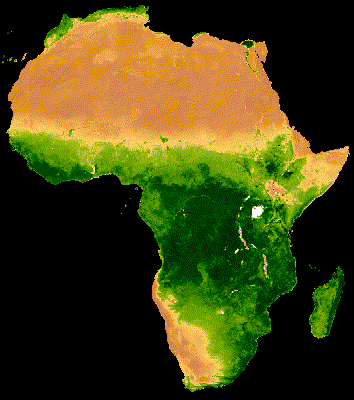
Visualization of the above collection shows considerable noise in the forested regions where cloud cover is heavy (Figure 2a). A better representation can be achieved by reducing serial date ranges by median across all years in the MODIS collection.
Code Editor (JavaScript)
// Make a day-of-year sequence from 1 to 365 with a 16-day step.
var doyList = ee.List.sequence(1, 365, 16);

// Import a MODIS NDVI collection.
var ndviCol = ee.ImageCollection('MODIS/006/MOD13A2').select('NDVI');

// Map over the list of days to build a list of image composites.
var ndviCompList = doyList.map(function(startDoy) {
  // Ensure that startDoy is a number.
  startDoy = ee.Number(startDoy);

  // Filter images by date range; starting with the current startDate and
  // ending 15 days later. Reduce the resulting image collection by median.
  return ndviCol
    .filter(ee.Filter.calendarRange(startDoy, startDoy.add(15), 'day_of_year'))
    .reduce(ee.Reducer.median());
});

// Convert the image List to an ImageCollection.
var ndviCompCol = ee.ImageCollection.fromImages(ndviCompList);
The animation resulting from this collection is less noisy, as each image represents the median of a 16-day NDVI composite for 20+ years of data (Figure 1b). See this tutorial for more information on this animation.
 |
 |
|---|---|
| Figure 2a. Annual NDVI without inter-annual compositing. | Figure 2b. Annual NDVI with inter-annual compositing. |
Intra-annual composite by filter and reduce
The previous example applies inter-annual compositing. It can also be helpful to composite a series of intra-annual observations. For example, Landsat data are collected every sixteen days for a given scene per sensor, but often some portion of the images are obscured by clouds. Masking out the clouds and compositing several images from the same season can produce a more cloud-free representation. Consider the following example where Landsat 5 images from July and August are composited using median for each year from 1985 to 2011.
Code Editor (JavaScript)
// Assemble a collection of Landsat surface reflectance images for a given
// region and day-of-year range.
var lsCol = ee.ImageCollection('LANDSAT/LT05/C02/T1_L2')
  .filterBounds(ee.Geometry.Point(-122.9, 43.6))
  .filter(ee.Filter.dayOfYear(182, 243))
  // Add the observation year as a property to each image.
  .map(function(img) {
    return img.set('year', ee.Image(img).date().get('year'));
  });


// Define a function to scale the data and mask unwanted pixels.
function maskL457sr(image) {
  // Bit 0 - Fill
  // Bit 1 - Dilated Cloud
  // Bit 2 - Unused
  // Bit 3 - Cloud
  // Bit 4 - Cloud Shadow
  var qaMask = image.select('QA_PIXEL').bitwiseAnd(parseInt('11111', 2)).eq(0);
  var saturationMask = image.select('QA_RADSAT').eq(0);

  // Apply the scaling factors to the appropriate bands.
  var opticalBands = image.select('SR_B.').multiply(0.0000275).add(-0.2);
  var thermalBand = image.select('ST_B6').multiply(0.00341802).add(149.0);

  // Replace the original bands with the scaled ones and apply the masks.
  return image.addBands(opticalBands, null, true)
      .addBands(thermalBand, null, true)
      .updateMask(qaMask)
      .updateMask(saturationMask);
}

// Define a list of unique observation years from the image collection.
var years = ee.List(lsCol.aggregate_array('year')).distinct().sort();

// Map over the list of years to build a list of annual image composites.
var lsCompList = years.map(function(year) {
  return lsCol
    // Filter image collection by year.
    .filterMetadata('year', 'equals', year)
    // Apply cloud mask.
    .map(maskL457sr)
    // Reduce image collection by median.
    .reduce(ee.Reducer.median())
    // Set composite year as an image property.
    .set('year', year);
});

// Convert the image List to an ImageCollection.
var lsCompCol = ee.ImageCollection.fromImages(lsCompList);
Intra-annual composite by join and reduce
Note that the previous two compositing methods map over a List of days and
years to incrementally define new dates to filter and composite over.
Applying a join is another method for achieving this operation. In the
following snippet, a unique year collection is defined and then a saveAll
join is applied to identify all images that correspond to a given year.
Images belonging to a given year are grouped into a List object which is
stored as a property of the respective year representative in the distinct
year collection. Annual composites are generated from these lists by reducing
ImageCollections defined by them in a function mapped over the distinct
year collection.
Code Editor (JavaScript)
// Assemble a collection of Landsat surface reflectance images for a given
// region and day-of-year range.
var lsCol = ee.ImageCollection('LANDSAT/LT05/C02/T1_L2')
  .filterBounds(ee.Geometry.Point(-122.9, 43.6))
  .filter(ee.Filter.dayOfYear(182, 243))
  // Add the observation year as a property to each image.
  .map(function(img) {
    return img.set('year', ee.Image(img).date().get('year'));
  });

// Make a distinct year collection; one image representative per year.
var distinctYears = lsCol.distinct('year').sort('year');

// Define a join filter; one-to-many join on ‘year’ property.
var filter = ee.Filter.equals({leftField: 'year', rightField: 'year'});

// Define a join.
var join = ee.Join.saveAll('year_match');

// Apply the join; results in 'year_match' property being added to each distinct
// year representative image. The list includes all images in the collection
// belonging to the respective year.
var joinCol = join.apply(distinctYears, lsCol, filter);

// Define a function to scale the data and mask unwanted pixels.
function maskL457sr(image) {
  // Bit 0 - Fill
  // Bit 1 - Dilated Cloud
  // Bit 2 - Unused
  // Bit 3 - Cloud
  // Bit 4 - Cloud Shadow
  var qaMask = image.select('QA_PIXEL').bitwiseAnd(parseInt('11111', 2)).eq(0);
  var saturationMask = image.select('QA_RADSAT').eq(0);

  // Apply the scaling factors to the appropriate bands.
  var opticalBands = image.select('SR_B.').multiply(0.0000275).add(-0.2);
  var thermalBand = image.select('ST_B6').multiply(0.00341802).add(149.0);

  // Replace the original bands with the scaled ones and apply the masks.
  return image.addBands(opticalBands, null, true)
      .addBands(thermalBand, null, true)
      .updateMask(qaMask)
      .updateMask(saturationMask);
}

// Map over the distinct years collection to build a list of annual image
// composites.
var lsCompList = joinCol.map(function(img) {
  // Get the list of images belonging to the given year.
  return ee.ImageCollection.fromImages(img.get('year_match'))
    // Apply cloud mask.
    .map(maskL457sr)
    // Reduce image collection by median.
    .reduce(ee.Reducer.median())
    // Set composite year as an image property.
    .copyProperties(img, ['year']);
});

// Convert the image List to an ImageCollection.
var lsCompCol = ee.ImageCollection(lsCompList);
Same-day composite by join and reduce
An additional case for compositing is to create spatially contiguous image mosaics. Suppose your region of interest spans two Landsat rows within the same path and your objective is to display an image mosaic of the two images for each Landsat 8 orbit in 2017 and 2018. Here, after filtering the collection by path and row, a join operation is used to mosaic Landsat images from the same obit, defined by acquisition date.
Code Editor (JavaScript)
var lsCol = ee.ImageCollection('LANDSAT/LC08/C02/T1_L2')
  .filterDate('2017-01-01', '2019-01-01')
  .filter('WRS_PATH == 38 && (WRS_ROW == 28 || WRS_ROW == 29)')
  .map(function(img) {
    var date = img.date().format('yyyy-MM-dd');
    return img.set('date', date);
  });

var distinctDates = lsCol.distinct('date').sort('date');
var filter = ee.Filter.equals({leftField: 'date', rightField: 'date'});
var join = ee.Join.saveAll('date_match');
var joinCol = join.apply(distinctDates, lsCol, filter);

var lsColMos = ee.ImageCollection(joinCol.map(function(col) {
  return ee.ImageCollection.fromImages(col.get('date_match')).mosaic();
}));
Sorting
Sort a collection by time to ensure proper chronological sequence, or order
by a property of your choice. By default, the visualization frame series is
sorted in natural order of the collection. The arrangement of the series can
be altered using the sort collection method, whereby an Image property is
selected for sorting in either ascending or descending order. For example, to
sort by time of observation, use the ubiquitous system:time_start property.
Code Editor (JavaScript)
var s2col = ee.ImageCollection('COPERNICUS/S2_SR')
  .filterBounds(ee.Geometry.Point(-122.1, 37.2))
  .sort('system:time_start');
Or perhaps the order should be defined by increasing cloudiness, as in this case of Sentinel-2 imagery.
Code Editor (JavaScript)
var s2col = ee.ImageCollection('COPERNICUS/S2_SR')
  .filterBounds(ee.Geometry.Point(-122.1, 37.2))
  .sort('CLOUDY_PIXEL_PERCENTAGE');
Order can also be defined by a derived property, such as mean regional NDVI. Here, regional NDVI is added as a property to each image in a mapped function, followed by a sort on the new property.
Code Editor (JavaScript)
// Define an area of interest geometry.
var aoi = ee.Geometry.Point(-122.1, 37.2).buffer(1e4);

// Filter MODIS NDVI image collection by a date range.
var ndviCol = ee.ImageCollection('MODIS/061/MOD13A1')
  .filterDate('2018-01-01', '2019-01-01')
  .select('NDVI')
  // Map over the image collection to calculate regional mean NDVI and add
  // the result to each image as a property.
  .map(function(img) {
    var meanNdvi = img.reduceRegion({
      reducer: ee.Reducer.mean(), geometry: aoi, scale: 500});
    return img.set('meanNdvi', meanNdvi.get('NDVI'));
  })
  // Sort the collection by descending regional mean NDVI.
  .sort('meanNdvi', false);
Image visualization
Image visualization transforms numbers into colors. There are three ways to control how image data are represented as color in collection visualization methods:
- Provide visualization arguments directly to
getVideoThumbURLandgetFilmstripThumbURL. - Map the
visualizeimage method over the image collection prior to application ofgetVideoThumbURLandgetFilmstripThumbURL. - Map the
sldStyleimage method over the image collection prior to application ofgetVideoThumbURLandgetFilmstripThumbURL. See Styled Layer Descriptor for more information.
The examples in this guide use options 1 and 2, where visualization is achieved by mapping three image bands of a multi-band image to color channels red, green, and blue or grading values of a single band linearly along a color palette. Visualization parameters include:
| Parameter | Description | Type |
|---|---|---|
| bands | Comma-delimited list of three band names to be mapped to RGB | list |
| min | Value(s) to map to 0 | number or list of three numbers, one for each band |
| max | Value(s) to map to 255 | number or list of three numbers, one for each band |
| gain | Value(s) by which to multiply each pixel value | number or list of three numbers, one for each band |
| bias | Value(s) to add to each DN | number or list of three numbers, one for each band |
| gamma | Gamma correction factor(s) | number or list of three numbers, one for each band |
| palette | List of CSS-style color strings (single-band images only) | comma-separated list of hex strings |
| opacity | The opacity of the layer (0.0 is fully transparent and 1.0 is fully opaque) | number |
Use the bands argument to select the band(s) you wish to visualize. Provide
a list of either one or three band names. With regard to multi-band images,
the first three bands are selected by default. Band name order determines
color assignment; the first, second, and third listed bands are mapped to
red, green, and blue, respectively.
Data range scaling is an important consideration when visualizing images. By
default, floating point data values between 0 and 1 (inclusive) are scaled
between 0 and 255 (inclusive). Values outside this range are forced to 0 and
255 depending on whether they are less than 0 or greater than 1,
respectively. With regard to integer data, the full capacity defined by its
type is scaled between 0 and 255 (e.g., signed 16-bit data has a range from
−32,768 to 32,767, which scales to [0, 255], by default). Accepting the
defaults can often result in visualizations with little to no contrast
between image features. Use min and max to improve contrast and emphasize
a particular data range. A good rule of thumb is to set min and max to
values that represent the 2nd and 98th percentile of the data within your
area of interest. See the following example of calculating these values for a
digital elevation model.
Code Editor (JavaScript)
// Import SRTM global elevation model.
var demImg = ee.Image('USGS/SRTMGL1_003');

// Define a rectangular area of interest.
var aoi = ee.Geometry.Polygon(
  [[
    [-103.84153083119054, 49.083004219142886],
    [-103.84153083119054, 25.06838270664608],
    [-85.64817145619054, 25.06838270664608],
    [-85.64817145619054, 49.083004219142886]
  ]],
  null, false);

// Calculate the 2nd and 98th percentile elevation values from rescaled (to
// 500m) pixels intersecting the area of interest. A Dictionary is returned.
var percentClip = demImg.reduceRegion({
  reducer: ee.Reducer.percentile([2, 98]),
  geometry: aoi,
  scale: 500,
  maxPixels: 3e7
});

// Print the regional 2nd and 98th percentile elevation values. Get the
// dictionary keys and use them to get the values for each percentile summary.
var keys = percentClip.keys();
print('Set vis min to:', ee.Number(percentClip.get(keys.get(0))).round());
print('Set vis max to:', ee.Number(percentClip.get(keys.get(1))).round());
The palette parameter defines the colors to represent the 8-bit
visualization image. It applies only to single-band representations;
specifying it with a multi-band image results in an error.
If the data are single-band or you would like to visualize a single band from
a multi-band image, set the forceRgbOutput parameter to true (unnecessary
if the palette argument is provided). Use the min and max parameters to
define the range of values to linearly scale between 0 and 255.
An example of mapping a visualization function over a single-band image
collection follows. A MODIS NDVI collection is imported, visualization
arguments for the visualization method are set, and a function that
transforms values into RGB image representations is mapped over the NDVI
collection.
Code Editor (JavaScript)
// Filter MODIS NDVI image collection by a date range.
var ndviCol = ee.ImageCollection('MODIS/061/MOD13A1')
  .filterDate('2018-01-01', '2019-01-01')
  .select('NDVI');

// Define visualization arguments.
var visArgs = {
  min: 0,
  max: 9000,
  palette: [
    'FFFFFF', 'CE7E45', 'DF923D', 'F1B555', 'FCD163', '99B718', '74A901',
    '66A000', '529400', '3E8601', '207401', '056201', '004C00', '023B01',
    '012E01', '011D01', '011301'
  ]
};

// Define a function to convert an image to an RGB visualization image and copy
// properties from the original image to the RGB image.
var visFun = function(img) {
  return img.visualize(visArgs).copyProperties(img, img.propertyNames());
};

// Map over the image collection to convert each image to an RGB visualization
// using the previously defined visualization function.
var ndviColVis = ndviCol.map(visFun);
Here is an example of mapping a visualization function over a multi-band image collection:
Code Editor (JavaScript)
// Assemble a collection of Sentinel-2 surface reflectance images for a given
// region and date range.
var s2col = ee.ImageCollection('COPERNICUS/S2_SR')
  .filterBounds(ee.Geometry.Point(-96.9037, 48.0395))
  .filterDate('2019-06-01', '2019-10-01');

// Define visualization arguments.
var visArgs = {bands: ['B11', 'B8', 'B3'], min: 300, max: 3500};

// Define a function to convert an image to an RGB visualization image and copy
// properties from the original image to the RGB image.
var visFun = function(img) {
  return img.visualize(visArgs).copyProperties(img, img.propertyNames());
};

// Map over the image collection to convert each image to an RGB visualization
// using the previously defined visualization function.
var s2colVis = s2col.map(visFun);
In this case, no palette argument is provided because three bands are given,
which define intensity for each RGB layer. Note that both examples use the
min and max parameters to control what values are stretched to the limits
of the 8-bit RGB data.
Video thumb
The getVideoThumbURL() function generates an animation from all images in
an ImageCollection where each image represents a frame. The general
workflow for producing an animation is as follows:
- Define a
Geometrywhose bounds determine the regional extent of the animation. - Define an
ImageCollection. - Consider image visualization: either map an image visualization function over the collection or add image visualization arguments to the set of animation arguments.
- Define animation arguments and call the
getVideoThumbURLmethod.
The result of getVideoThumbURL is a URL. Print the URL to the console and
click it to start Earth Engine servers generating the animation on-the-fly in
a new browser tab. Alternatively, view the animation in the Code Editor
console by calling the ui.Thumbnail function on the collection and its
corresponding animation arguments. Upon rendering, the animation is available
for downloading by right clicking on it and selecting appropriate options
from its context menu.
The following example illustrates generating an animation depicting global
temperatures over the course of 24 hours. Note that this example includes
visualization arguments along with animation arguments, as opposed to first
mapping a visualization function over the ImageCollection. Upon running
this script, an animation similar to Figure 3 should appear in the Code
Editor console.
Code Editor (JavaScript)
// Define an area of interest geometry with a global non-polar extent.
var aoi = ee.Geometry.Polygon(
  [[[-179.0, 78.0], [-179.0, -58.0], [179.0, -58.0], [179.0, 78.0]]], null,
  false);

// Import hourly predicted temperature image collection for northern winter
// solstice. Note that predictions extend for 384 hours; limit the collection
// to the first 24 hours.
var tempCol = ee.ImageCollection('NOAA/GFS0P25')
  .filterDate('2018-12-22', '2018-12-23')
  .limit(24)
  .select('temperature_2m_above_ground');

// Define arguments for animation function parameters.
var videoArgs = {
  dimensions: 768,
  region: aoi,
  framesPerSecond: 7,
  crs: 'EPSG:3857',
  min: -40.0,
  max: 35.0,
  palette: ['blue', 'purple', 'cyan', 'green', 'yellow', 'red']
};

// Print the animation to the console as a ui.Thumbnail using the above defined
// arguments. Note that ui.Thumbnail produces an animation when the first input
// is an ee.ImageCollection instead of an ee.Image.
print(ui.Thumbnail(tempCol, videoArgs));

// Alternatively, print a URL that will produce the animation when accessed.
print(tempCol.getVideoThumbURL(videoArgs));
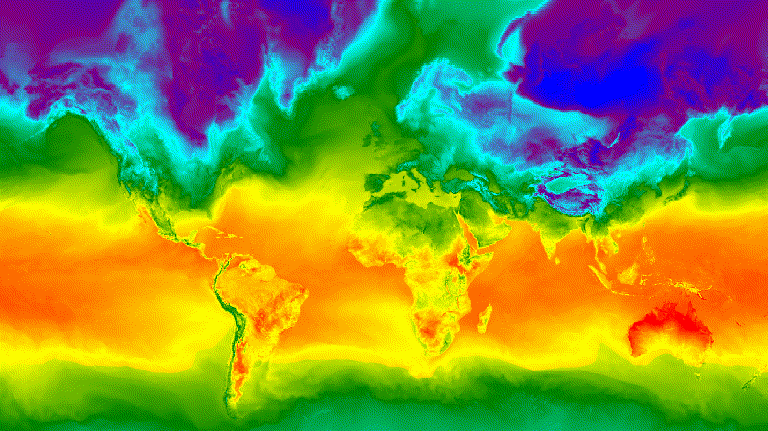
Figure 3. Hourly surface temperature for the northern winter solstice
represented as an animated GIF image.
Filmstrip
The getFilmstripThumbUrl function generates a single static image
representing the concatenation of all images in an ImageCollection into a
north-south series. The sequence of filmstrip frames follow the natural order
of the collection.
The result of getFilmstripThumbUrl is a URL. Print the URL to the console
and click it to start Earth Engine servers generating the image on-the-fly in
a new browser tab. Upon rendering, the image is available for downloading by
right clicking on it and selecting appropriate options from its context menu.
The following code snippet uses the same collection as the video thumb example above. Upon running this script, a filmstrip similar to Figure 4 should appear in the Code Editor console.
Code Editor (JavaScript)
// Define an area of interest geometry with a global non-polar extent.
var aoi = ee.Geometry.Polygon(
  [[[-179.0, 78.0], [-179.0, -58.0], [179.0, -58.0], [179.0, 78.0]]], null,
  false);

// Import hourly predicted temperature image collection for northern winter
// solstice. Note that predictions extend for 384 hours; limit the collection
// to the first 24 hours.
var tempCol = ee.ImageCollection('NOAA/GFS0P25')
  .filterDate('2018-12-22', '2018-12-23')
  .limit(24)
  .select('temperature_2m_above_ground');

// Define arguments for the getFilmstripThumbURL function parameters.
var filmArgs = {
  dimensions: 128,
  region: aoi,
  crs: 'EPSG:3857',
  min: -40.0,
  max: 35.0,
  palette: ['blue', 'purple', 'cyan', 'green', 'yellow', 'red']
};

// Print a URL that will produce the filmstrip when accessed.
print(tempCol.getFilmstripThumbURL(filmArgs));
![]()
Figure 4. Hourly surface temperature for the northern winter solstice
represented as a filmstrip PNG image. Note that the filmstrip has been
divided into four sections for display; the result of getFilmstripThumbURL
is a single series of collection images joined north-south.
Advanced techniques
The following sections describe how to use clipping, opacity, and layer compositing to enhance visualizations by adding polygon borders, emphasizing regions of interest, and comparing images within a collection.
Note that all of the following examples in this section use the same base
ImageCollection defined here:
Code Editor (JavaScript)
// Import hourly predicted temperature image collection for northern winter
// solstice. Note that predictions extend for 384 hours; limit the collection
// to the first 24 hours.
var tempCol = ee.ImageCollection('NOAA/GFS0P25')
  .filterDate('2018-12-22', '2018-12-23')
  .limit(24)
  .select('temperature_2m_above_ground');

// Define visualization arguments to control the stretch and color gradient
// of the data.
var visArgs = {
  min: -40.0,
  max: 35.0,
  palette: ['blue', 'purple', 'cyan', 'green', 'yellow', 'red']
};

// Convert each image to an RGB visualization image by mapping the visualize
// function over the image collection using the arguments defined previously.
var tempColVis = tempCol.map(function(img) {
  return img.visualize(visArgs);
});

// Import country features and filter to South American countries.
var southAmCol = ee.FeatureCollection('USDOS/LSIB_SIMPLE/2017')
  .filterMetadata('wld_rgn', 'equals', 'South America');

// Define animation region (South America with buffer).
var southAmAoi = ee.Geometry.Rectangle({
  coords: [-103.6, -58.8, -18.4, 17.4], geodesic: false});
Overlays
Multiple images can be overlaid using the blend Image method where
overlapping pixels from two images are blended based on their masks (opacity).
Vector overlay
Adding administrative boundary polygons and other geometries to an image can provide valuable spatial context. Consider the global daily surface temperature animation above (Figure 3). The boundaries between land and ocean are somewhat discernible, but they can be made explicit by adding a polygon overlay of countries.
Vector data (Features) are drawn to images by applying the paint method.
Features can be painted to an existing image, but the better practice is to
paint them to a blank image, style it, and then blend the result with other
styled image layers. Treating each layer of a visualization stack
independently affords more control over styling.
The following example demonstrates painting South American country borders to
a blank Image and blending the result with each Image of the global daily
temperature collection (Figure 5). The overlaid country boundaries
distinguish land from water and provide context to patterns of temperature.
Code Editor (JavaScript)
// Define an empty image to paint features to.
var empty = ee.Image().byte();

// Paint country feature edges to the empty image.
var southAmOutline = empty
  .paint({featureCollection: southAmCol, color: 1, width: 1})
  // Convert to an RGB visualization image; set line color to black.
  .visualize({palette: '000000'});

// Map a blend operation over the temperature collection to overlay the country
// border outline image on all collection images.
var tempColOutline = tempColVis.map(function(img) {
  return img.blend(southAmOutline);
});

// Define animation arguments.
var videoArgs = {
  dimensions: 768,
  region: southAmAoi,
  framesPerSecond: 7,
  crs: 'EPSG:3857'
};

// Display the animation.
print(ui.Thumbnail(tempColOutline, videoArgs));
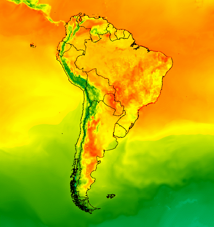
Figure 5. Add vector overlays to images in a collection to provide spatial context.
Image overlay
Several images can be overlaid to achieve a desired style. Suppose you want to emphasize a region of interest. You can create a muted copy of an image visualization as a base layer and then overlay a clipped version of the original visualization. Building on the previous example, the following script produces Figure 6.
Code Editor (JavaScript)
// Define an empty image to paint features to.
var empty = ee.Image().byte();

// Paint country feature edges to the empty image.
var southAmOutline = empty
  .paint({featureCollection: southAmCol, color: 1, width: 1})
  // Convert to an RGB visualization image; set line color to black.
  .visualize({palette: '000000'});

// Map a blend operation over the temperature collection to overlay the country
// border outline image on all collection images.
var tempColOutline = tempColVis.map(function(img) {
  return img.blend(southAmOutline);
});

// Define a partially opaque grey RGB image to dull the underlying image when
// blended as an overlay.
var dullLayer = ee.Image.constant(175).visualize({
  opacity: 0.6, min: 0, max: 255, forceRgbOutput: true});

// Map a two-part blending operation over the country outline temperature
// collection for final styling.
var finalVisCol = tempColOutline.map(function(img) {
  return img
    // Blend the dulling layer with the given country outline temperature image.
    .blend(dullLayer)
    // Blend a clipped copy of the country outline temperature image with the
    // dulled background image.
    .blend(img.clipToCollection(southAmCol));
});

// Define animation arguments.
var videoArgs = {
  dimensions: 768,
  region: southAmAoi,
  framesPerSecond: 7,
  crs: 'EPSG:3857'
};

// Display the animation.
print(ui.Thumbnail(finalVisCol, videoArgs));
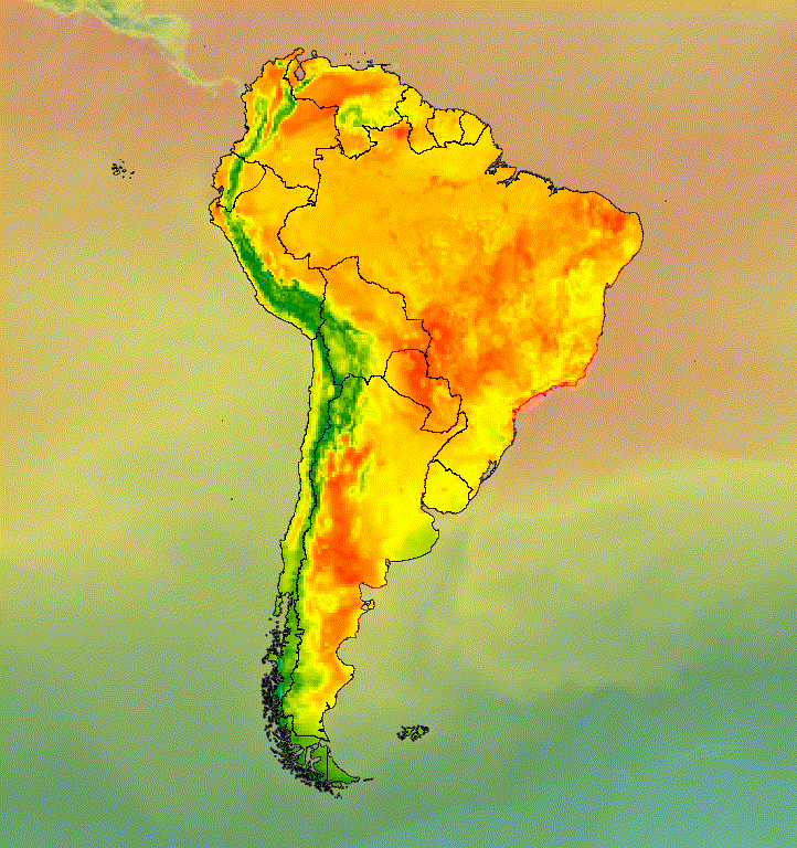
Figure 6. Emphasize an area of interest by clipping the image and overlaying
it on a muted copy.
You can also blend image data with a hillshade base layer to indicate terrain and give the visualization some depth (Figure 7).
Code Editor (JavaScript)
// Define a hillshade layer from SRTM digital elevation model.
var hillshade = ee.Terrain.hillshade(ee.Image('USGS/SRTMGL1_003')
  // Exaggerate the elevation to increase contrast in hillshade.
  .multiply(100))
  // Clip the DEM by South American boundary to clean boundary between
  // land and ocean.
  .clipToCollection(southAmCol);

// Map a blend operation over the temperature collection to overlay a partially
// opaque temperature layer on the hillshade layer.
var finalVisCol = tempColVis.map(function(img) {
  return hillshade
    .blend(img.clipToCollection(southAmCol).visualize({opacity: 0.6}));
});

// Define animation arguments.
var videoArgs = {
  dimensions: 768,
  region: southAmAoi,
  framesPerSecond: 7,
  crs: 'EPSG:3857'
};

// Display the animation.
print(ui.Thumbnail(finalVisCol, videoArgs));
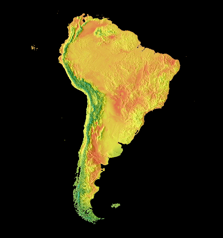
Figure 7. Show terrain by overlaying partially transparent image data on a
hillshade layer.
Transitions
Customize an image collection to produce animations that reveal differences between two images within a collection using fade, flicker, and slide transitions. Each of the following examples use the same base visualization generated by the following script:
Code Editor (JavaScript)
// Define an area of interest geometry with a global non-polar extent.
var aoi = ee.Geometry.Polygon(
  [[[-179.0, 78.0], [-179.0, -58.0], [179.0, -58.0], [179.0, 78.0]]], null,
  false);

// Import hourly predicted temperature image collection.
var temp = ee.ImageCollection('NOAA/GFS0P25')

// Define a northern summer solstice temperature image.
var summerSolTemp = temp
  .filterDate('2018-06-21', '2018-06-22')
  .filterMetadata('forecast_hours', 'equals', 12)
  .first()
  .select('temperature_2m_above_ground');

// Define a northern winter solstice temperature image.
var winterSolTemp = temp
  .filterDate('2018-12-22', '2018-12-23')
  .filterMetadata('forecast_hours', 'equals', 12)
  .first()
  .select('temperature_2m_above_ground');

// Combine the solstice images into a collection.
var tempCol = ee.ImageCollection([
  summerSolTemp.set('season', 'summer'),
  winterSolTemp.set('season', 'winter')
]);

// Import international boundaries feature collection.
var countries = ee.FeatureCollection('USDOS/LSIB_SIMPLE/2017');

// Define visualization arguments.
var visArgs = {
  min: -40.0,
  max: 35.0,
  palette: ['blue', 'purple', 'cyan', 'green', 'yellow', 'red']
};

// Convert the image data to RGB visualization images.
// The clip and unmask combination sets ocean pixels to black.
var tempColVis = tempCol.map(function(img) {
  return img
    .visualize(visArgs)
    .clipToCollection(countries)
    .unmask(0)
    .copyProperties(img, img.propertyNames());
});
Flicker
With only two images in a collection, as is the case here, flicker is the
default representation upon collection animation. Adjust the
framesPerSecond animation argument to speed up or slow down the flicker
rate. The following visualization arguments applied to the collection above
produces Figure 8.
Code Editor (JavaScript)
// Define arguments for animation function parameters.
var videoArgs = {
  dimensions: 768,
  region: aoi,
  framesPerSecond: 2,
  crs: 'EPSG:3857'
};

// Display animation to the Code Editor console.
print(ui.Thumbnail(tempColVis, videoArgs));
Figure 8. Example of flickering between 12pm GMT surface temperature for
northern and winter solstice.
Fade
A fade transition between two layers is achieved by simultaneously decreasing the opacity of one layer while increasing the opacity of the other over a sequence of opacity increments from near 0 to 1 (Figure 9).
Code Editor (JavaScript)
// Define a sequence of decreasing opacity increments. Note that opacity cannot
// be 0, so near 1 and 0 are used. Near 1 is needed because a compliment is
// calculated in a following step that can result in 0 if 1 is an element of the
// list.
var opacityList = ee.List.sequence({start: 0.99999, end: 0.00001, count: 20});

// Filter the summer and winter solstice images from the collection and set as
// image objects.
var summerImg = tempColVis.filter(ee.Filter.eq('season', 'summer')).first();
var winterImg = tempColVis.filter(ee.Filter.eq('season', 'winter')).first();

// Map over the list of opacity increments to iteratively adjust the opacity of
// the two solstice images. Returns a list of images.
var imgList = opacityList.map(function(opacity) {
  var opacityCompliment = ee.Number(1).subtract(ee.Number(opacity));
  var winterImgFade = winterImg.visualize({opacity: opacity});
  var summerImgFade = summerImg.visualize({opacity: opacityCompliment});
  return summerImgFade.blend(winterImgFade).set('opacity', opacity);
});

// Convert the image list to an image collection; the forward phase.
var fadeForward = ee.ImageCollection.fromImages(imgList);

// Make a copy of the collection that is sorted by ascending opacity to
// represent the reverse phase.
var fadeBackward = fadeForward.sort({property: 'opacity'});

// Merge the forward and reverse phase frame collections.
var fadeCol = fadeForward.merge(fadeBackward);

// Define animation arguments.
var videoArgs = {
  dimensions: 768,
  region: aoi,
  framesPerSecond: 25,
  crs: 'EPSG:3857'
};

// Display the animation.
print(ui.Thumbnail(fadeCol, videoArgs));
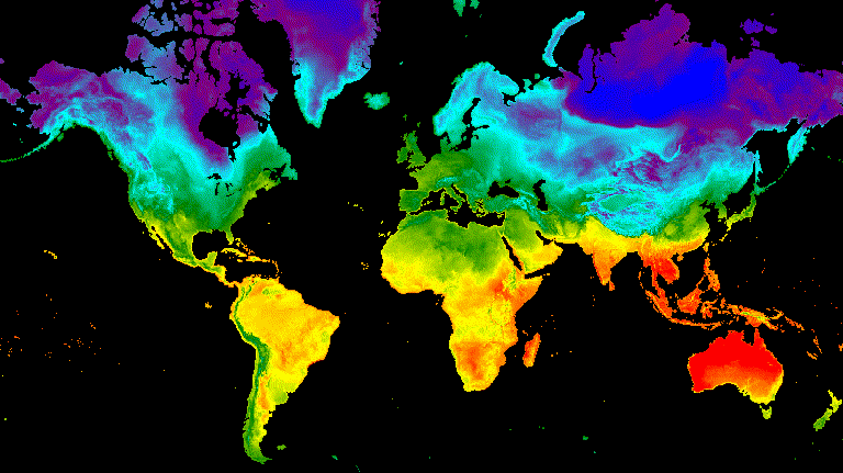
Figure 9. Example of fading between 12pm GMT surface temperature for summer
and winter solstice.
Slider
A slider transition progressively shows and hides the underlying image layer. It is achieved by iteratively adjusting the opacity of the overlying image across a range of longitudes (Figure 10).
Code Editor (JavaScript)
// Define a sequence of longitude increments. Start and end are defined by the
// min and max longitude of the feature to be provided to the region parameter
// of the animation arguments dictionary.
var lonSeq = ee.List.sequence({start: -179, end: 179, count: 20});

// Define a longitude image.
var longitude = ee.Image.pixelLonLat().select('longitude');

// Filter the summer and winter solstice images from the collection and set as
// image objects.
var summerImg = tempColVis.filter(ee.Filter.eq('season', 'summer')).first();
var winterImg = tempColVis.filter(ee.Filter.eq('season', 'winter')).first();

// Map over the list of longitude increments to iteratively adjust the mask
// (opacity) of the overlying image layer. Returns a list of images.
var imgList = lonSeq.map(function(lon) {
  lon = ee.Number(lon);
  var mask = longitude.gt(lon);
  return summerImg.blend(winterImg.updateMask(mask)).set('lon', lon);
});

// Convert the image list to an image collection; concealing phase.
var sliderColForward = ee.ImageCollection.fromImages(imgList);

// Make a copy of the collection that is sorted by descending longitude to
// represent the revealing phase.
var sliderColbackward = sliderColForward
  .sort({property: 'lon', ascending: false});

// Merge the forward and backward phase frame collections.
var sliderCol = sliderColForward.merge(sliderColbackward);

// Define animation arguments.
var videoArgs = {
  dimensions: 768,
  region: aoi,
  framesPerSecond: 25,
  crs: 'EPSG:3857'
};

// Display the animation.
print(ui.Thumbnail(sliderCol, videoArgs));

Figure 10. Example of a sliding transition between 12pm GMT surface temperature
for summer and winter solstice.