 GitHub でソースを見る
ee.Image オブジェクトには、意思決定式を構築するための一連のリレーショナル メソッド、条件付きメソッド、ブール値メソッドがあります。これらの方法の結果は、マスク、分類マップの開発、値の再割り当てによって、特定のピクセルまたは領域に分析を制限する場合に役立ちます。
関係演算子とブール演算子
リレーショナル メソッドには、次のようなものがあります。
eq()、gt()、gte()、lt()、lte()
ブール値メソッドには次のものがあります。
コードエディタ(JavaScript)
and()、or()、not()
Colab(Python)
And()、Or()、Not()
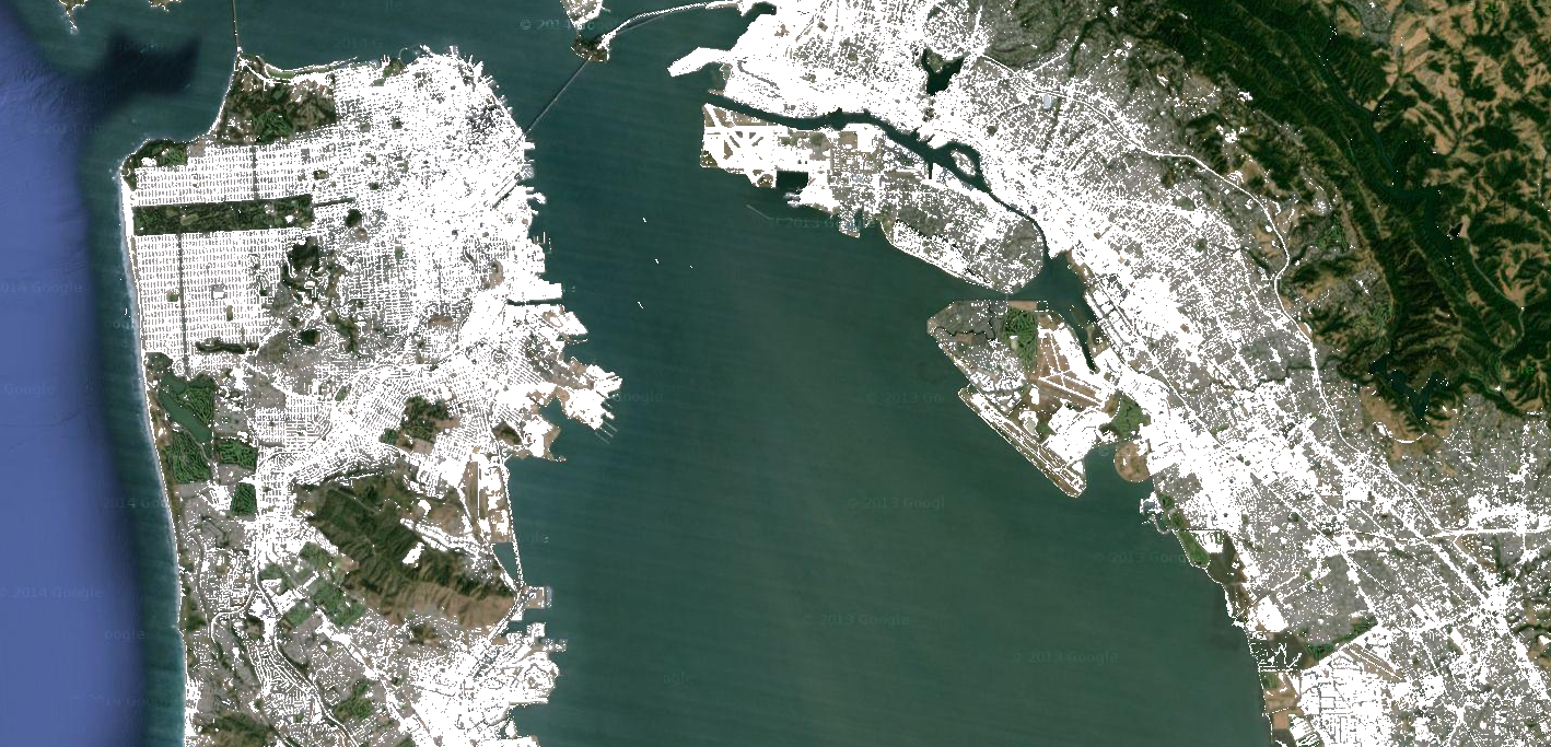
画像間のピクセル単位の比較を行うには、関係演算子を使用します。画像内の都市化地域を抽出するには、この例では関係演算子を使用してスペクトル指標をしきい値に設定し、しきい値を and 演算子と組み合わせます。
コードエディタ(JavaScript)
// Load a Landsat 8 image.
var image = ee.Image('LANDSAT/LC08/C02/T1_TOA/LC08_044034_20140318');

// Create NDVI and NDWI spectral indices.
var ndvi = image.normalizedDifference(['B5', 'B4']);
var ndwi = image.normalizedDifference(['B3', 'B5']);

// Create a binary layer using logical operations.
var bare = ndvi.lt(0.2).and(ndwi.lt(0));

// Mask and display the binary layer.
Map.setCenter(-122.3578, 37.7726, 12);
Map.setOptions('satellite');
Map.addLayer(bare.selfMask(), {}, 'bare');
import ee
import geemap.core as geemap
Colab(Python)
# Load a Landsat 8 image.
image = ee.Image('LANDSAT/LC08/C02/T1_TOA/LC08_044034_20140318')

# Create NDVI and NDWI spectral indices.
ndvi = image.normalizedDifference(['B5', 'B4'])
ndwi = image.normalizedDifference(['B3', 'B5'])

# Create a binary layer using logical operations.
bare = ndvi.lt(0.2).And(ndwi.lt(0))

# Define a map centered on San Francisco Bay.
map_bare = geemap.Map(center=[37.7726, -122.3578], zoom=12)

# Add the masked image layer to the map and display it.
map_bare.add_layer(bare.selfMask(), None, 'bare')
display(map_bare)
この例に示すように、関係演算子とブール演算子の出力は、true(1)または false(0)のいずれかです。0 をマスクするには、selfMask() を使用して、結果のバイナリ画像を自身でマスクします。
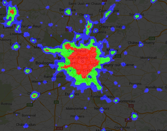
関係演算子とブール演算子によって返されるバイナリ画像は、数学演算子で使用できます。この例では、関係演算子と add() を使用して、夜間照明画像に都市化ゾーンを作成します。
コードエディタ(JavaScript)
// Load a 2012 nightlights image.
var nl2012 = ee.Image('NOAA/DMSP-OLS/NIGHTTIME_LIGHTS/F182012');
var lights = nl2012.select('stable_lights');

// Define arbitrary thresholds on the 6-bit stable lights band.
var zones = lights.gt(30).add(lights.gt(55)).add(lights.gt(62));

// Display the thresholded image as three distinct zones near Paris.
var palette = ['000000', '0000FF', '00FF00', 'FF0000'];
Map.setCenter(2.373, 48.8683, 8);
Map.addLayer(zones, {min: 0, max: 3, palette: palette}, 'development zones');
import ee
import geemap.core as geemap
Colab(Python)
# Load a 2012 nightlights image.
nl_2012 = ee.Image('NOAA/DMSP-OLS/NIGHTTIME_LIGHTS/F182012')
lights = nl_2012.select('stable_lights')

# Define arbitrary thresholds on the 6-bit stable lights band.
zones = lights.gt(30).add(lights.gt(55)).add(lights.gt(62))

# Define a map centered on Paris, France.
map_zones = geemap.Map(center=[48.8683, 2.373], zoom=8)

# Display the thresholded image as three distinct zones near Paris.
palette = ['000000', '0000FF', '00FF00', 'FF0000']
map_zones.add_layer(
    zones, {'min': 0, 'max': 3, 'palette': palette}, 'development zones'
)
display(map_zones)
条件演算子
上の例のコードは、expression() で実装された三項演算子を使用する場合と同じです。
コードエディタ(JavaScript)
// Create zones using an expression, display.
var zonesExp = nl2012.expression(
    "(b('stable_lights') > 62) ? 3" +
      ": (b('stable_lights') > 55) ? 2" +
        ": (b('stable_lights') > 30) ? 1" +
          ": 0"
);
Map.addLayer(zonesExp,
             {min: 0, max: 3, palette: palette},
             'development zones (ternary)');
import ee
import geemap.core as geemap
Colab(Python)
# Create zones using an expression, display.
zones_exp = nl_2012.expression(
    "(b('stable_lights') > 62) ? 3 "
    ": (b('stable_lights') > 55) ? 2 "
    ": (b('stable_lights') > 30) ? 1 "
    ': 0'
)

# Define a map centered on Paris, France.
map_zones_exp = geemap.Map(center=[48.8683, 2.373], zoom=8)

# Add the image layer to the map and display it.
map_zones_exp.add_layer(
    zones_exp, {'min': 0, 'max': 3, 'palette': palette}, 'zones exp'
)
display(map_zones_exp)
前の式の例では、関心のあるバンドは変数名の辞書ではなく、b() 関数を使用して参照されています。画像式の詳細については、こちらのページをご覧ください。数学演算子または式を使用すると、同じ結果が得られます。
画像に条件付きオペレーションを実装する別の方法として、where() 演算子を使用することもできます。マスキングされたピクセルを他のデータに置き換える必要があるかどうかを検討します。次の例では、where() を使用して、雲の多いピクセルが雲のない画像のピクセルに置き換えられます。
コードエディタ(JavaScript)
// Load a cloudy Sentinel-2 image.
var image = ee.Image(
  'COPERNICUS/S2_SR/20210114T185729_20210114T185730_T10SEG');
Map.addLayer(image,
             {bands: ['B4', 'B3', 'B2'], min: 0, max: 2000},
             'original image');

// Load another image to replace the cloudy pixels.
var replacement = ee.Image(
  'COPERNICUS/S2_SR/20210109T185751_20210109T185931_T10SEG');

// Set cloudy pixels (greater than 5% probability) to the other image.
var replaced = image.where(image.select('MSK_CLDPRB').gt(5), replacement);

// Display the result.
Map.setCenter(-122.3769, 37.7349, 11);
Map.addLayer(replaced,
             {bands: ['B4', 'B3', 'B2'], min: 0, max: 2000},
             'clouds replaced');
import ee
import geemap.core as geemap
Colab(Python)
# Load a cloudy Sentinel-2 image.
image = ee.Image('COPERNICUS/S2_SR/20210114T185729_20210114T185730_T10SEG')

# Load another image to replace the cloudy pixels.
replacement = ee.Image(
    'COPERNICUS/S2_SR/20210109T185751_20210109T185931_T10SEG'
)

# Set cloudy pixels (greater than 5% probability) to the other image.
replaced = image.where(image.select('MSK_CLDPRB').gt(5), replacement)

# Define a map centered on San Francisco Bay.
map_replaced = geemap.Map(center=[37.7349, -122.3769], zoom=11)

# Display the images on a map.
vis_params = {'bands': ['B4', 'B3', 'B2'], 'min': 0, 'max': 2000}
map_replaced.add_layer(image, vis_params, 'original image')
map_replaced.add_layer(replaced, vis_params, 'clouds replaced')
display(map_replaced)