An Intro to the Earth Engine Python API

Author(s): guiattard

Within the last decade, a large amount of geospatial data, such as satellite data (e.g. land surface temperature, vegetation) or the output of large scale, even global models (e.g. wind speed, groundwater recharge), have become freely available from multiple national agencies and universities (e.g. NASA, USGS, NOAA, and ESA). These geospatial data are used every day by scientists and engineers of all fields, to predict weather, prevent disasters, secure water supply, or study the consequences of climate change. When using these geospatial data, a few questions arise:

What data are available and where can it be found?
How can we access these data?
How can we manipulate these petabytes of data?

In this tutorial, an introduction to the Google Earth Engine Python API is presented. After some setup and some exploration of the Earth Engine Data Catalog, we’ll see how to handle geospatial datasets with pandas and make some plots with matplotlib.

First, we’ll see how to get the timeseries of a variable for a region of interest. An application of this procedure will be done to extract land surface temperature in an urban and a rural area near the city of Lyon, France to illustrate the heat island effect. Secondly, we will detail procedures for static mapping and exporting results as a GeoTIFF.

Finally, the folium library will be introduced to make interactive maps. In this last part, we’ll see how to include some GEE datasets as tile layers of a folium map.

Exploration of the Earth Engine Data Catalog

Have you ever thought that getting a meteorological dataset could be as easy as finding the nearest pizzeria? To convince you, visit the Earth Engine Data Catalog and explore datasets using the search bar or browsing by tag.

Let's say that we need to know the elevation of a region, some soil properties (e.g. clay, sand, silt content) and some meteorological observations (e.g. temperature, precipitation, evapotranspiration). Well, inside the Earth Engine Catalog we find:

SRTM global elevation with a resolution of 30 m,
OpenLandMap datasets with soil properties at a resolution of 250 m (e.g. clay, sand, and silt content), and
GRIDMET temperature, precipitation, and evapotranspiration, for example.

Of course the resolution, frequency, spatial and temporal extent, as well as data source (e.g. satellite image, interpolated station data, or model output) vary from one dataset to another. Therefore, read the description carefully and make sure you know what kind of dataset you are selecting!

Run me first

First of all, run the following cell to initialize the API. The output will contain instructions on how to grant this notebook access to Earth Engine using your account.

import ee

# Trigger the authentication flow.
ee.Authenticate()

# Initialize the library.
ee.Initialize(project='my-project')

Getting started with Collections

In the Earth Engine Data Catalog, datasets can be of different types:

Features which are geometric objects with a list of properties. For example, a watershed with some properties such as name and area, is an ee.Feature.
Images which are like features, but may include several bands. For example, the ground elevation given by the USGS here is an ee.Image.
Collections which are groups of features or images. For example, the Global Administrative Unit Layers giving administrative boundaries is a ee.FeatureCollection and the MODIS Land Surface Temperature dataset is an ee.ImageCollection.

If you want to know more about different data models, you may want to visit the Earth Engine User Guide.

In the following sections, we work with the MODIS land cover (LC), the MODIS land surface temperature (LST) and with the USGS ground elevation (ELV), which are ee.ImageCollections. The dataset descriptions provide us with all the information we need to import and manipulate these datasets: the availability, the provider, the Earth Engine Snippet, and the available bands associated with images in the collection.

Now, to import the LC, LST and ELV collections, we can copy and paste the Earth Engine Snippets:

# Import the MODIS land cover collection.
lc = ee.ImageCollection('MODIS/006/MCD12Q1')

# Import the MODIS land surface temperature collection.
lst = ee.ImageCollection('MODIS/006/MOD11A1')

# Import the USGS ground elevation image.
elv = ee.Image('USGS/SRTMGL1_003')

/tmpfs/src/tf_docs_env/lib/python3.9/site-packages/ee/deprecation.py:207: DeprecationWarning: 

Attention required for MODIS/006/MCD12Q1! You are using a deprecated asset.
To ensure continued functionality, please update it.
Learn more: https://developers.google.com/earth-engine/datasets/catalog/MODIS_006_MCD12Q1

  warnings.warn(warning, category=DeprecationWarning)
/tmpfs/src/tf_docs_env/lib/python3.9/site-packages/ee/deprecation.py:207: DeprecationWarning: 

Attention required for MODIS/006/MOD11A1! You are using a deprecated asset.
To ensure continued functionality, please update it.
Learn more: https://developers.google.com/earth-engine/datasets/catalog/MODIS_006_MOD11A1

  warnings.warn(warning, category=DeprecationWarning)

All of these images come in a different resolution, frequency, and possibly projection, ranging from daily images in a 1 km resolution for LST (hence an ee.ImageCollection — a collection of several ee.Images) to a single image representing data for the year 2000 in a 30 m resolution for the ELV. While we need to have an eye on the frequency, GEE takes care of resolution and projection by resampling and reprojecting all data we are going to work with to a common projection (learn more about projections in Earth Engine). We can define the resolution (called scale in GEE) whenever necessary and of course have the option to force no reprojection.

As you can see in the description of the datasets, they include several sets of information stored in several bands. For example, these bands are associated with the LST collection:

LST_Day_1km: Daytime Land Surface Temperature
Day_view_time: Local time of day observation
LST_Night_1km: Nighttime Land Surface Temperature
etc.

The description page of the collection tells us that the name of the band associated with the daytime LST is LST_Day_1km which is in units of Kelvin. In addition, values are ranging from 7,500 to 65,535 with a corrective scale of 0.02.

Then, we have to filter the collection on the period of time we want. We can do that using the filterDate() method. We also need to select the bands we want to work with. Therefore, we decide to focus on daytime LST so we select the daytime band LST_Day_1km and its associated quality indicator QC_Day with the select() method.

# Initial date of interest (inclusive).
i_date = '2017-01-01'

# Final date of interest (exclusive).
f_date = '2020-01-01'

# Selection of appropriate bands and dates for LST.
lst = lst.select('LST_Day_1km', 'QC_Day').filterDate(i_date, f_date)

Now, we can either upload existing shape files or define some points with longitude and latitude coordinates where we want to know more about LC, LST and ELV. For this example, let's use two point locations:

The first one in the urban area of Lyon, France
The second one, 30 kilometers away from the city center, in a rural area

# Define the urban location of interest as a point near Lyon, France.
u_lon = 4.8148
u_lat = 45.7758
u_poi = ee.Geometry.Point(u_lon, u_lat)

# Define the rural location of interest as a point away from the city.
r_lon = 5.175964
r_lat = 45.574064
r_poi = ee.Geometry.Point(r_lon, r_lat)

We can easily get information about our region/point of interest using the following methods (to get more information about available methods and required arguments, please visit the API documentation here):

sample(): samples the image (does NOT work for an ee.ImageCollection — we'll talk about sampling an ee.ImageCollection later) according to a given geometry and a scale (in meters) of the projection to sample in. It returns an ee.FeatureCollection.
first(): returns the first entry of the collection,
get(): to select the appropriate band of your Image/Collection,
getInfo(): evaluates server-side expression graph and transfers result to client.

Then we can query the ground elevation and LST around our point of interest using the following commands. Please be careful when evaluating LST. According to the dataset description, the value should be corrected by a factor of 0.02 to get units of Kelvin (do not forget the conversion). To get the mean multi-annual daytime LST, we use the mean() collection reduction method on the LST ee.ImageCollection. (The following run might take about 15-20 seconds)

scale = 1000  # scale in meters

# Print the elevation near Lyon, France.
elv_urban_point = elv.sample(u_poi, scale).first().get('elevation').getInfo()
print('Ground elevation at urban point:', elv_urban_point, 'm')

# Calculate and print the mean value of the LST collection at the point.
lst_urban_point = lst.mean().sample(u_poi, scale).first().get('LST_Day_1km').getInfo()
print('Average daytime LST at urban point:', round(lst_urban_point*0.02 -273.15, 2), '°C')

# Print the land cover type at the point.
lc_urban_point = lc.first().sample(u_poi, scale).first().get('LC_Type1').getInfo()
print('Land cover value at urban point is:', lc_urban_point)

Ground elevation at urban point: 196 m
Average daytime LST at urban point: 23.12 °C
Land cover value at urban point is: 13

Going back to the band description of the lc dataset, we see that a lc value of "13" corresponds to an urban land. You can run the above cells with the rural point coordinates if you want to notice a difference.

Get a time series

Now that you see we can get geospatial information about a place of interest pretty easily, you may want to inspect a time series, probably make some charts and calculate statistics about a place. Hence, we import the data at the given locations using the getRegion() method.

# Get the data for the pixel intersecting the point in urban area.
lst_u_poi = lst.getRegion(u_poi, scale).getInfo()

# Get the data for the pixel intersecting the point in rural area.
lst_r_poi = lst.getRegion(r_poi, scale).getInfo()

# Preview the result.
lst_u_poi[:5]

[['id', 'longitude', 'latitude', 'time', 'LST_Day_1km', 'QC_Day'],
 ['2017_01_01', 4.810478346460038, 45.77365530231022, 1483228800000, None, 2],
 ['2017_01_02', 4.810478346460038, 45.77365530231022, 1483315200000, None, 2],
 ['2017_01_03', 4.810478346460038, 45.77365530231022, 1483401600000, None, 2],
 ['2017_01_04',
  4.810478346460038,
  45.77365530231022,
  1483488000000,
  13808,
  17]]

Printing the first 5 lines of the result shows that we now have arrays full of data. As we can see several None values appear in the LST_Day_1km column. The associated quality indicator QC_Day indicates a value of 2 meaning that the LST is not calculated because of cloud effects.

We now define a function to transform this array into a pandas Dataframe which is much more convenient to manipulate.

import pandas as pd

def ee_array_to_df(arr, list_of_bands):
    """Transforms client-side ee.Image.getRegion array to pandas.DataFrame."""
    df = pd.DataFrame(arr)

    # Rearrange the header.
    headers = df.iloc[0]
    df = pd.DataFrame(df.values[1:], columns=headers)

    # Remove rows without data inside.
    df = df[['longitude', 'latitude', 'time', *list_of_bands]].dropna()

    # Convert the data to numeric values.
    for band in list_of_bands:
        df[band] = pd.to_numeric(df[band], errors='coerce')

    # Convert the time field into a datetime.
    df['datetime'] = pd.to_datetime(df['time'], unit='ms')

    # Keep the columns of interest.
    df = df[['time','datetime',  *list_of_bands]]

    return df

We apply this function to get the two time series we want (and print one).

lst_df_urban = ee_array_to_df(lst_u_poi,['LST_Day_1km'])

def t_modis_to_celsius(t_modis):
    """Converts MODIS LST units to degrees Celsius."""
    t_celsius =  0.02*t_modis - 273.15
    return t_celsius

# Apply the function to get temperature in celsius.
lst_df_urban['LST_Day_1km'] = lst_df_urban['LST_Day_1km'].apply(t_modis_to_celsius)

# Do the same for the rural point.
lst_df_rural = ee_array_to_df(lst_r_poi,['LST_Day_1km'])
lst_df_rural['LST_Day_1km'] = lst_df_rural['LST_Day_1km'].apply(t_modis_to_celsius)

lst_df_urban.head()

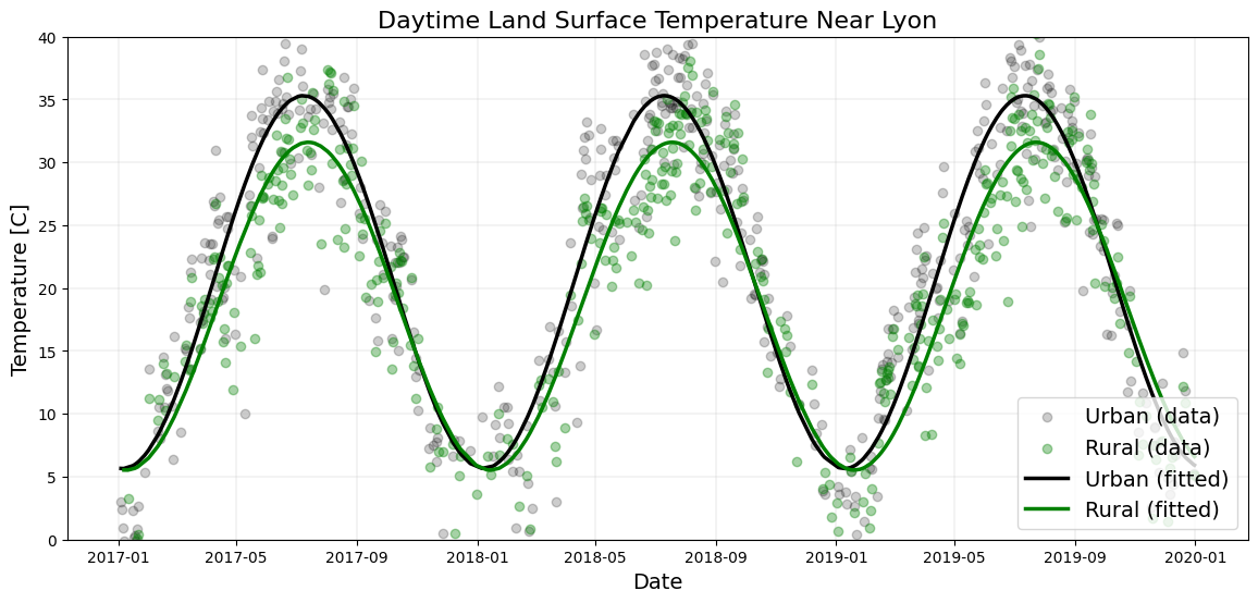
Now that we have our data in a good shape, we can easily make plots and compare the trends. As the area of Lyon, France experiences a semi-continental climate, we expect that LST has a seasonality influence and the sinusoidal trend described by Stallman (1965) reading as follow:

$$ LST(t) = LST_{0} + \frac{\Delta _{LST}}{2}sin(\frac{2\pi t}{\tau} + \phi) $$

where:

$LST_{0}$ represents the mean annual LST,
$\Delta _{LST}$ represents the amplitude between maximal and minimal LST,
$\tau$ represents the period of oscillation of LST, and
$\phi$ represents an offset needed to adjust the time when $LST(t) = LST_{0}$

Consequently, on the top of the data scatter plot, we plot the fitting curve using the scipy library:

import matplotlib.pyplot as plt
import numpy as np
from scipy import optimize
%matplotlib inline

# Fitting curves.
## First, extract x values (times) from the dfs.
x_data_u = np.asanyarray(lst_df_urban['time'].apply(float))  # urban
x_data_r = np.asanyarray(lst_df_rural['time'].apply(float))  # rural

## Secondly, extract y values (LST) from the dfs.
y_data_u = np.asanyarray(lst_df_urban['LST_Day_1km'].apply(float))  # urban
y_data_r = np.asanyarray(lst_df_rural['LST_Day_1km'].apply(float))  # rural

## Then, define the fitting function with parameters.
def fit_func(t, lst0, delta_lst, tau, phi):
    return lst0 + (delta_lst/2)*np.sin(2*np.pi*t/tau + phi)

## Optimize the parameters using a good start p0.
lst0 = 20
delta_lst = 40
tau = 365*24*3600*1000   # milliseconds in a year
phi = 2*np.pi*4*30.5*3600*1000/tau  # offset regarding when we expect LST(t)=LST0

params_u, params_covariance_u = optimize.curve_fit(
    fit_func, x_data_u, y_data_u, p0=[lst0, delta_lst, tau, phi])
params_r, params_covariance_r = optimize.curve_fit(
    fit_func, x_data_r, y_data_r, p0=[lst0, delta_lst, tau, phi])

# Subplots.
fig, ax = plt.subplots(figsize=(14, 6))

# Add scatter plots.
ax.scatter(lst_df_urban['datetime'], lst_df_urban['LST_Day_1km'],
           c='black', alpha=0.2, label='Urban (data)')
ax.scatter(lst_df_rural['datetime'], lst_df_rural['LST_Day_1km'],
           c='green', alpha=0.35, label='Rural (data)')

# Add fitting curves.
ax.plot(lst_df_urban['datetime'],
        fit_func(x_data_u, params_u[0], params_u[1], params_u[2], params_u[3]),
        label='Urban (fitted)', color='black', lw=2.5)
ax.plot(lst_df_rural['datetime'],
        fit_func(x_data_r, params_r[0], params_r[1], params_r[2], params_r[3]),
        label='Rural (fitted)', color='green', lw=2.5)

# Add some parameters.
ax.set_title('Daytime Land Surface Temperature Near Lyon', fontsize=16)
ax.set_xlabel('Date', fontsize=14)
ax.set_ylabel('Temperature [C]', fontsize=14)
ax.set_ylim(-0, 40)
ax.grid(lw=0.2)
ax.legend(fontsize=14, loc='lower right')

plt.show()

png

Static mapping of land surface temperature and ground elevation

Get a static map

Now, we want to get static maps of land surface temperature and ground elevation around a region of interest. We define this region of interest using a buffer zone of 1000 km around Lyon, France.

# Define a region of interest with a buffer zone of 1000 km around Lyon.
roi = u_poi.buffer(1e6)

Also, we have to convert the LST ee.ImageCollection into an ee.Image, for example by taking the mean value of each pixel over the period of interest. And we convert the value of pixels into Celsius:

# Reduce the LST collection by mean.
lst_img = lst.mean()

# Adjust for scale factor.
lst_img = lst_img.select('LST_Day_1km').multiply(0.02)

# Convert Kelvin to Celsius.
lst_img = lst_img.select('LST_Day_1km').add(-273.15)

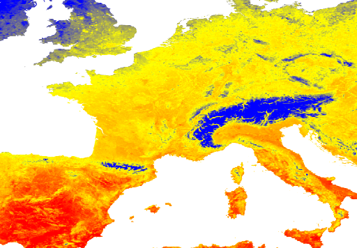
Then, we use the getThumbUrl() method to get a URL and we can use the IPython library to display the mean daytime LST map for the region of interest. Blue represents the coldest areas (< 10°C) and red represents the warmest areas (> 30°C) (note that it may take a moment for the image to load after the cell completes execution).

from IPython.display import Image

# Create a URL to the styled image for a region around France.
url = lst_img.getThumbUrl({
    'min': 10, 'max': 30, 'dimensions': 512, 'region': roi,
    'palette': ['blue', 'yellow', 'orange', 'red']})
print(url)

# Display the thumbnail land surface temperature in France.
print('\nPlease wait while the thumbnail loads, it may take a moment...')
Image(url=url)

https://earthengine.googleapis.com/v1/projects/earthengine-legacy/thumbnails/3bc4413e4552eae1fc382b446c52ce06-432bbb7e7e3cf35ffe3d5210b4015c48:getPixels

Please wait while the thumbnail loads, it may take a moment...

png

We do the same for ground elevation:

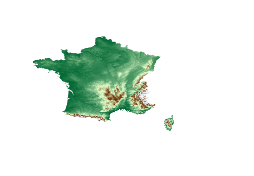
# Make pixels with elevation below sea level transparent.
elv_img = elv.updateMask(elv.gt(0))

# Display the thumbnail of styled elevation in France.
Image(url=elv_img.getThumbURL({
    'min': 0, 'max': 2000, 'dimensions': 512, 'region': roi,
    'palette': ['006633', 'E5FFCC', '662A00', 'D8D8D8', 'F5F5F5']}))

png

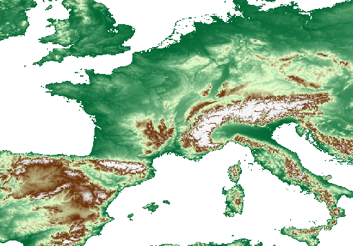
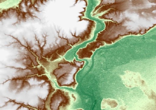
Of course you may want to have a closer look around a specific part of the map. So let's define another region (a buffer zone around Lyon), adjust the min/max scale and display:

# Create a buffer zone of 10 km around Lyon.
lyon = u_poi.buffer(10000)  # meters

url = elv_img.getThumbUrl({
    'min': 150, 'max': 350, 'region': lyon, 'dimensions': 512,
    'palette': ['006633', 'E5FFCC', '662A00', 'D8D8D8', 'F5F5F5']})
Image(url=url)

jpeg

Clip an image by a region of interest

In case you want to display an image over a given region (and not outside), we can clip our dataset using the region as an argument of the clip() method. Let's say that we want to display the ground elevation in France. We can get the geometry of the administrative boundary of France with the FAO feature collection and do the same as before:

# Get a feature collection of administrative boundaries.
countries = ee.FeatureCollection('FAO/GAUL/2015/level0').select('ADM0_NAME')

# Filter the feature collection to subset France.
france = countries.filter(ee.Filter.eq('ADM0_NAME', 'France'))

# Clip the image by France.
elv_fr = elv_img.clip(france)

# Create the URL associated with the styled image data.
url = elv_fr.getThumbUrl({
    'min': 0, 'max': 2500, 'region': roi, 'dimensions': 512,
    'palette': ['006633', 'E5FFCC', '662A00', 'D8D8D8', 'F5F5F5']})

# Display a thumbnail of elevation in France.
Image(url=url)

png

Export a GeoTIFF file

After manipulating Earth Engine datasets, you may need to export a resulting ee.Image to a GeoTIFF. For example, to use it as an input of a numerical model outside of Earth Engine, or to overlap it with personal georeferenced files in your favorite GIS. There are multiple ways to do that (see the Exporting section of the Developer Guide). Here we explore two options:

Save the ee.Image you want in Google Drive
Directly download the image.

Save a GeoTIFF file in your Google Drive

To export the ee.Image to Google Drive, we have to define a task and start it. We have to specify the size of pixels (here 30 m), the projection (here EPSG:4326), the file format (here GeoTIFF), the region of interest (here the area of Lyon defined before), and the file will be exported to the Google Drive directory head and named according to the fileNamePrefix we choose.

task = ee.batch.Export.image.toDrive(image=elv_img,
                                     description='elevation_near_lyon_france',
                                     scale=30,
                                     region=lyon,
                                     fileNamePrefix='my_export_lyon',
                                     crs='EPSG:4326',
                                     fileFormat='GeoTIFF')
task.start()

Then we can check the status of our task (note: the task will also be registered in the JavaScript Code Editor's list of tasks) using the status() method. Depending on the size of the request, we might run this cell several times until the task state becomes 'COMPLETED' (in order, the state of the export task is 'READY', then 'RUNNING', and finally 'COMPLETED').

task.status()

{'state': '...',
 'description': 'Placeholder status - run notebook for real output',
 'creation_timestamp_ms': 1647567508236,
 'update_timestamp_ms': 1647567508236,
 'start_timestamp_ms': 0,
 'task_type': '...',
 'id': '...',
 'name': '...'}

Now you can check your google drive to find your file.

Get a link to download your GeoTIFF

Similarly, we can use the getDownloadUrl() method and click on the provided link. Please note the following points:

For large or long-running exports, using the ee.batch.Export module (previous section) is a better method.
The token to generate the Earth Engine layer tiles expires after about a day.

link = lst_img.getDownloadURL({
    'scale': 30,
    'crs': 'EPSG:4326',
    'fileFormat': 'GeoTIFF',
    'region': lyon})
print(link)

https://earthengine.googleapis.com/v1/projects/earthengine-legacy/thumbnails/c56be60a3910586fa7b35913fa6cfe3c-0a79426b0dbfe36321a9c39014c4c5b4:getPixels

Interactive mapping using folium

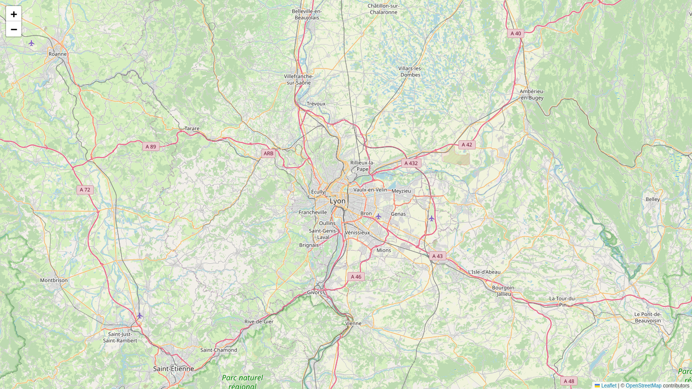
To display these GEE datasets on an interactive map, let me introduce you to folium. Folium is a python library based on leaflet.js (open-source JavaScript library for mobile-friendly interactive maps) that you can use to make interactive maps. Folium supports WMS, GeoJSON layers, vector layers, and tile layers which make it very convenient and straightforward to visualize the data we manipulate with python. We create our first interactive map with one line of code, specifying the location where we want to center the map, the zoom level, and the main dimensions of the map:

import folium

# Define the center of our map.
lat, lon = 45.77, 4.855

my_map = folium.Map(location=[lat, lon], zoom_start=10)
my_map

png

On top of this map, we now want to add the GEE layers we studied before: land cover (LC), land surface temperature (LST) and ground elevation model (ELV). For each GEE dataset, the process consists of adding a new tile layer to our map with specified visualization parameters. Let's define a new method for handing Earth Engine tiles and using it to display an elevation model to a Leaflet map.

def add_ee_layer(self, ee_image_object, vis_params, name):
    """Adds a method for displaying Earth Engine image tiles to folium map."""
    map_id_dict = ee.Image(ee_image_object).getMapId(vis_params)
    folium.raster_layers.TileLayer(
        tiles=map_id_dict['tile_fetcher'].url_format,
        attr='Map Data &copy; <a href="https://earthengine.google.com/">Google Earth Engine</a>',
        name=name,
        overlay=True,
        control=True
    ).add_to(self)

# Add Earth Engine drawing method to folium.
folium.Map.add_ee_layer = add_ee_layer

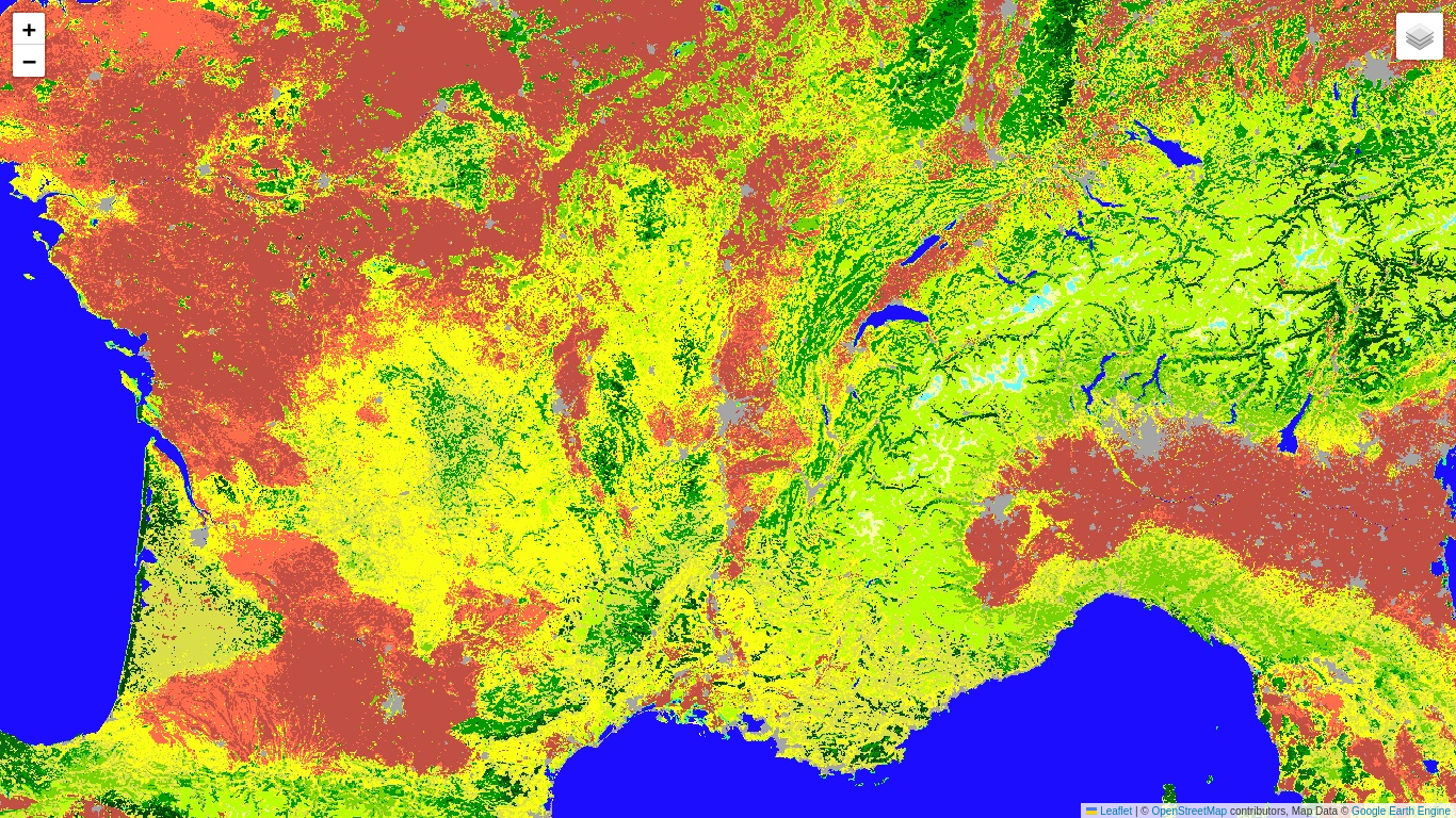
We want to respect the common LC classes defined in the table of the previous section (hexadecimal codes are given for each class: water bodies are blue, urban areas are grey, forests are green, etc.). Then we define visualization parameters associated with LC and apply the method we defined earlier:

# Select a specific band and dates for land cover.
lc_img = lc.select('LC_Type1').filterDate(i_date).first()

# Set visualization parameters for land cover.
lc_vis_params = {
    'min': 1,'max': 17,
    'palette': ['05450a','086a10', '54a708', '78d203', '009900', 'c6b044',
                'dcd159', 'dade48', 'fbff13', 'b6ff05', '27ff87', 'c24f44',
                'a5a5a5', 'ff6d4c', '69fff8', 'f9ffa4', '1c0dff']
}

# Create a map.
lat, lon = 45.77, 4.855
my_map = folium.Map(location=[lat, lon], zoom_start=7)

# Add the land cover to the map object.
my_map.add_ee_layer(lc_img, lc_vis_params, 'Land Cover')

# Add a layer control panel to the map.
my_map.add_child(folium.LayerControl())

# Display the map.
display(my_map)

png

Finally, the map can be saved in HTML format using the folium method save() specifying the file name as an argument of this method. If you run this cell using Google Colab, your HTML file is saved in the content folder of your Colab environment. If you run this cell locally, the file is saved inside your current working directory. Then, you will be able to open your HTML file with your favorite navigator.

my_map.save('my_lc_interactive_map.html')

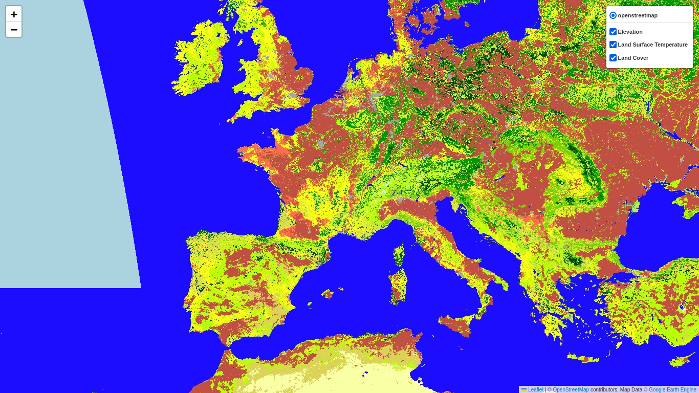
Of course we can add other datasets similarly, by defining some visualization parameters and by adding the appropriate tiles:

# Set visualization parameters for ground elevation.
elv_vis_params = {
    'min': 0, 'max': 4000,
    'palette': ['006633', 'E5FFCC', '662A00', 'D8D8D8', 'F5F5F5']}

# Set visualization parameters for land surface temperature.
lst_vis_params = {
    'min': 0, 'max': 40,
    'palette': ['white', 'blue', 'green', 'yellow', 'orange', 'red']}

# Arrange layers inside a list (elevation, LST and land cover).
ee_tiles = [elv_img, lst_img, lc_img]

# Arrange visualization parameters inside a list.
ee_vis_params = [elv_vis_params, lst_vis_params, lc_vis_params]

# Arrange layer names inside a list.
ee_tiles_names = ['Elevation', 'Land Surface Temperature', 'Land Cover']

# Create a new map.
lat, lon = 45.77, 4.855
my_map = folium.Map(location=[lat, lon], zoom_start=5)

# Add layers to the map using a loop.
for tile, vis_param, name in zip(ee_tiles, ee_vis_params, ee_tiles_names):
    my_map.add_ee_layer(tile, vis_param, name)

folium.LayerControl(collapsed = False).add_to(my_map)

my_map

png

Documentation

The full documentation of the Google Earth Engine Python API is available here.
The Google Earth Engine User Guide is available here.
Some tutorials are available here.
An example based on the Google Earth Engine Javascript console dedicated to Land Surface Temperature estimation is provided in the open access supplementary material of Benz et al., (2017). You can access the code here.

Acknowledgements

Thanks to Susanne Benz and Justin Braaten for reviewing and helping write this tutorial.