Page Summary
-
This tutorial analyzes Sentinel-1 SAR imagery to detect statistically significant changes on the Earth's surface, requiring an understanding of SAR image statistical properties and hypothesis testing fundamentals.
-
Sentinel-1 images in the GEE archive, in IW mode, have pixels averaged over 5 looks in the range direction and resampled to 10x10 m^2, resulting in an effective number of looks of approximately 4.4.
-
The intensity values of single-look complex SAR images have an exponential distribution, while multi-look intensity images follow a gamma distribution, with the variance decreasing inversely with the number of looks.
-
The equivalent number of looks (ENL) for Sentinel-1 IW mode imagery is approximately 4.4, calculated as the square of the mean divided by the variance of the intensity values in a textureless area.
 View source on GitHub
In this tutorial we will analyze synthetic aperture radar (SAR) imagery in order to detect statistically significant changes on the Earth surface. As the adverb "statistically" hints, we will need a basic understanding of the statistical properties of SAR imagery in order to proceed, and the adjective "significant" implies that we learn the fundamentals of hypothesis testing. In particular we will be concerned with time series of the dual polarimetric intensity Sentinel-1 SAR images in the GEE archive. The tutorial is in four parts:
- 1. Single and multi-look image statistics
- 2. Hypothesis testing
- 3. Multitemporal change detection
- 4. Applications
Much of the material is based on Chapters 5 and 9 of my text Image Analysis, Classification and Change Detection in Remote Sensing, and the most relevant original publications are Conradsen et al. (2003), Conradsen et al. (2016) and Canty et al. (2020). For those more interested in the theoretical background and/or less comfortable with the Python API, see the monograph "Detecting Changes in Synthetic Aperture Radar Imager"
Context
The Sentinel-1 missions of the ESA provide a fantastic source of weather-independent, day-or-night Earth observation data with repeat times of the order of 6 days. The Google Earth Engine team monitor and ingest the imagery data almost as fast as they are produced, thus removing the burden from the user of searching, downloading, pre-processing and georeferencing. The JavaScript and Python API's to GEE can then be easily programmed to analyze time series of Sentinel-1 acquisitions virtually anywhere on the globe. Detected changes, both short- and long-term, can be related to landscape dynamics and human activity.
Prerequisites
A basic knowledge of the Sentinel-1 SAR platform is assumed on the part of the reader, at the level of the ESA User Guides. The reader should also be familiar with ordinary Python syntax and also with the GEE API (Python or JavaScript, it doesn't matter as they are almost identical). We will take a relaxed view of statistical formalism, without clearly distinguishing random variables from their realizations (measurements). We assume that the reader has, at least, an intuitive understanding of the mean and variance of independent measurements \(x_i\) of a quantity \(x\),
and that the measurements can be described by a probability density function \(p(x)\) with
and
More statistics will be introduced as needed. A highly recommended reference is Freund's Mathematical Statistics.
Part 1. Single and multi-look image statistics
Run me first
Run the following cell to initialize the API. The output will contain instructions on how to grant this notebook access to Earth Engine using your account.
import ee

# Trigger the authentication flow.
ee.Authenticate()

# Initialize the library.
ee.Initialize(project='my-project')
Datasets and Python modules
Two datasets will be used in the tutorial:
COPERNICUS/S1_GRD_FLOAT
- Sentinel-1 ground range detected images
COPERNICUS/S1_GRD
- Sentinel-1 ground range detected images converted to decibels
The following cell imports some python modules which we will be using as we go along, and also enables inline graphics.
import matplotlib.pyplot as plt
import numpy as np
from scipy.stats import norm, gamma, f, chi2
import IPython.display as disp
%matplotlib inline
And in order to make use of interactive maps, we import the folium package:
# Import the Folium library.
import folium
# Define a method for displaying Earth Engine image tiles to folium map.
def add_ee_layer(self, ee_image_object, vis_params, name):
map_id_dict = ee.Image(ee_image_object).getMapId(vis_params)
folium.raster_layers.TileLayer(
tiles = map_id_dict['tile_fetcher'].url_format,
attr = 'Map Data © <a href="https://earthengine.google.com/">Google Earth Engine</a>',
name = name,
overlay = True,
control = True
).add_to(self)
# Add EE drawing method to folium.
folium.Map.add_ee_layer = add_ee_layer
A Sentinel-1 image
Let's start work by grabbing a spatial subset of a Sentinel-1 image from the archive. We'll define an region of interest (AOI) as the long-lat corners of a rectangle over the Frankfurt Airport. A convenient way to do this is with the geojson.io website, from which we can cut and paste the corresponding GeoJSON object description.
geoJSON = {
  "type": "FeatureCollection",
  "features": [
    {
      "type": "Feature",
      "properties": {},
      "geometry": {
        "type": "Polygon",
        "coordinates": [
          [
            [
              8.473892211914062,
              49.98081240937428
            ],
            [
              8.658599853515625,
              49.98081240937428
            ],
            [
              8.658599853515625,
              50.06066538593667
            ],
            [
              8.473892211914062,
              50.06066538593667
            ],
            [
              8.473892211914062,
              49.98081240937428
            ]
          ]
        ]
      }
    }
  ]
}
Note that the last and first corners are identical, indicating closure of the polygon. We have to bore down into the GeoJSON structure to get the geometry coordinates, then create an ee.Geometry() object:
coords = geoJSON['features'][0]['geometry']['coordinates']
aoi = ee.Geometry.Polygon(coords)
Next, we filter the S1 archive to get an image over the aoi acquired sometime in August, 2020. Any old image will do fine, so we won't bother to specify the orbit number or whether we want the ASCENDING or DESCENDING node. If we don't specify the instrument mode or resolution, we get IW (interferometric wide swath) mode and \(10\times 10\ m^2\) pixels by default. For convenience we grab both decibel and float versions:
ffa_db = ee.Image(ee.ImageCollection('COPERNICUS/S1_GRD')
                       .filterBounds(aoi)
                       .filterDate(ee.Date('2020-08-01'), ee.Date('2020-08-31'))
                       .first()
                       .clip(aoi))
ffa_fl = ee.Image(ee.ImageCollection('COPERNICUS/S1_GRD_FLOAT')
                       .filterBounds(aoi)
                       .filterDate(ee.Date('2020-08-01'), ee.Date('2020-08-31'))
                       .first()
                       .clip(aoi))
Notice that we have clipped the images to our aoi so as not to work with the entire swath. To confirm that we have an image, we list its band names, fetching the result from the GEE servers with the getInfo() class method:
ffa_db.bandNames().getInfo()
['VV', 'VH', 'angle']
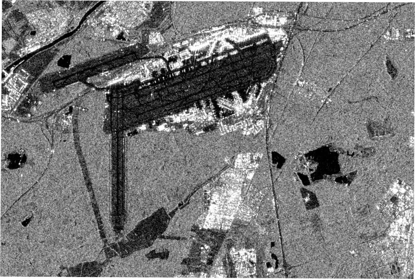
and display the VV band of the decibel version using the getThumbURL() method and IPython's display module. The float intensities \(I\) are generally between 0 and 1, so we stretch the decibel image \(10\log_{10}(I)\) from \(-20\) to \(0\):
url = ffa_db.select('VV').getThumbURL({'min': -20, 'max': 0})
disp.Image(url=url, width=800)
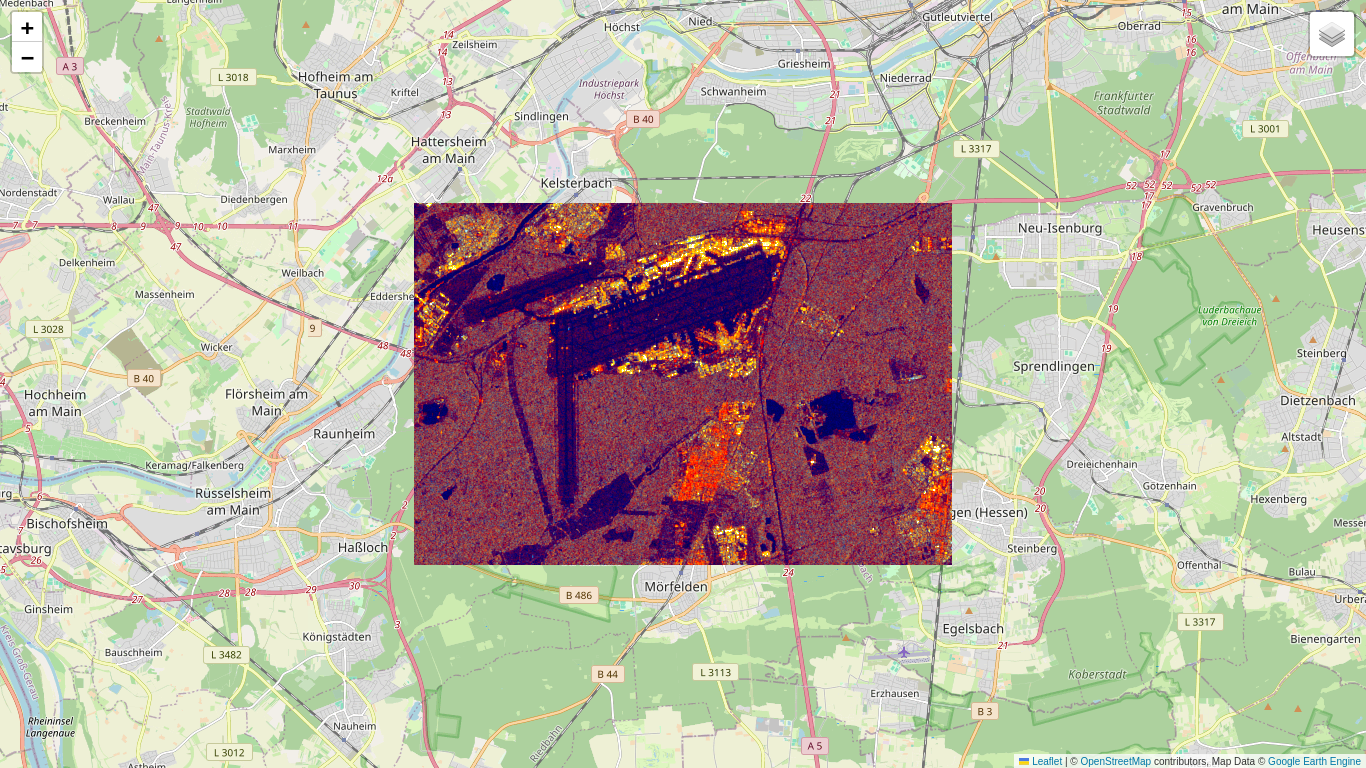
This is fine, but a little boring. We can use folium to project onto a map for geographical context. The folium Map() constructor wants its location keyword in long-lat rather than lat-long, so we do a list reverse in the first line:
location = aoi.centroid().coordinates().getInfo()[::-1]

# Make an RGB color composite image (VV,VH,VV/VH).
rgb = ee.Image.rgb(ffa_db.select('VV'),
                   ffa_db.select('VH'),
                   ffa_db.select('VV').divide(ffa_db.select('VH')))

# Create the map object.
m = folium.Map(location=location, zoom_start=12)

# Add the S1 rgb composite to the map object.
m.add_ee_layer(rgb, {'min': [-20, -20, 0], 'max': [0, 0, 2]}, 'FFA')

# Add a layer control panel to the map.
m.add_child(folium.LayerControl())

# Display the map.
display(m)
Pixel distributions
In order to examine the statistics of the pixels in this image empirically, we'll need samples from a featureless (textureless) spatial subset. Here is a polygon covering the triangular wooded area just east of the north-south runway:
geoJSON = {
  "type": "FeatureCollection",
  "features": [
    {
      "type": "Feature",
      "properties": {},
      "geometry": {
        "type": "Polygon",
        "coordinates": [
          [
            [
              8.534317016601562,
              50.021637833966786
            ],
            [
              8.530540466308594,
              49.99780882512238
            ],
            [
              8.564186096191406,
              50.00663576154257
            ],
            [
              8.578605651855469,
              50.019431940583104
            ],
            [
              8.534317016601562,
              50.021637833966786
            ]
          ]
        ]
      }
    }
  ]
}
coords = geoJSON['features'][0]['geometry']['coordinates']
aoi_sub = ee.Geometry.Polygon(coords)
Using standard reducers from the GEE library we can easily calculate a histogram and estimate the first two moments (mean and variance) of the pixels in the polygon aoi_sub , again retrieving the results from the servers with getInfo() .
hist = ffa_fl.select('VV').reduceRegion(
    ee.Reducer.fixedHistogram(0, 0.5, 500),aoi_sub).get('VV').getInfo()
mean = ffa_fl.select('VV').reduceRegion(
    ee.Reducer.mean(), aoi_sub).get('VV').getInfo()
variance = ffa_fl.select('VV').reduceRegion(
    ee.Reducer.variance(), aoi_sub).get('VV').getInfo()
Here is a plot of the (normalized) histogram using numpy and matplotlib :
a = np.array(hist)
x = a[:, 0]                 # array of bucket edge positions
y = a[:, 1]/np.sum(a[:, 1]) # normalized array of bucket contents
plt.grid()
plt.plot(x, y, '.')
plt.show()
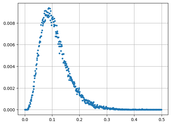
The above histogram is in fact a gamma probability density distribution
where
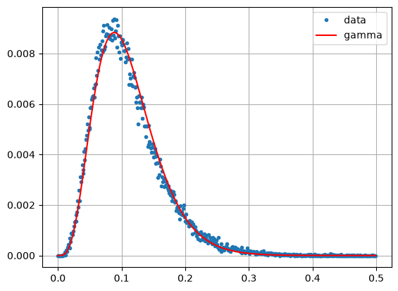
The parameters are in this case \(\alpha = 5\) and \(\beta = {\mu}/\alpha\), where \(\mu\) is the estimated mean value we just determined with ee.Reducer.mean(). This can easily be verified by plotting the gamma distribution gamma.pdf() and overlaying it onto the histogram. Since the bucket widths are 0.001, we have to divide the plot by 1000.
alpha = 5
beta = mean/alpha
plt.grid()
plt.plot(x, y, '.', label='data')
plt.plot(x, gamma.pdf(x, alpha, 0, beta)/1000, '-r', label='gamma')
plt.legend()
plt.show()
In order to understand just why this is the case, let's take a step back and consider how the pixels were generated.
Single look complex (SLC) SAR measurements
The Sentinel-1 platform is a dual polarimetric synthetic aperture radar system, emitting radar microwaves in the C-band with one polarization (vertical in most cases) and recording both vertical and horizontal reflected polarizations. This is represented mathematically as
The incident, vertically polarized radar signal \(\pmatrix{E_v^i\cr 0}\) is transformed by a complex scattering matrix \(\pmatrix{S_{vv} & S_{vh}\cr S_{hv} & S_{hh}}\) into the backscattered signal \(\pmatrix{E_v^b\cr E_h^b}\) having both vertical and horizontal polarization components. The exponent term accounts for the phase shift due to the return distance \(r\) from target to sensor, where \(k\) is the wave number, \(k=2\pi/\lambda\). From measurement of the backscattered radiation at the sensor, two of the four complex scattering matrix elements can be derived and processed into two-dimensional (slant range \(\times\) azimuth) arrays, comprising the so-called single look complex image. Written as a complex vector, the two derived elements are
We write the complex transpose of the vector \(S\) as \(S^\dagger = (S_{vv}^*\ S_{vh}^*)\), where the \(^*\) denotes complex conjugation. The inner product of \(S\) with itself is the total power (also referred to as the span image)
and the outer product is the (dual pol) covariance matrix image
The diagonal elements are real numbers, the off-diagonal elements are complex conjugates of each other and contain the relative phases of the \(S_{vv}\) and \(S_{vh}\) components. The off-diagonal elements are not available for S1 archived imagery in GEE, so that if we nevertheless choose to represent the data in covariance matrix form, the matrix is diagonal:
In terms of radar scattering cross sections (sigma nought),
Speckle
The most striking characteristic of SAR images, when compared to their visual/infrared counterparts, is the disconcerting speckle effect which makes visual interpretation very difficult. Speckle gives the appearance of random noise, but it is actually a deterministic consequence of the coherent nature of the radar signal.
For single polarization transmission and reception, e.g., vertical-vertical (\(vv\)), the received SLC signal can be modelled in the form
where \(|S^a_{vv}|\) is the overall amplitude characterizing the signal scattered from the area covered by a single pixel, e.g., \(10\times 10\ m^2\) for our S1 data, with the phase set equal to zero for convenience. The effects of randomly distributed scatterers within the irradiated area, with dimensions of the order of the incident wavelength 5.6 cm (for Sentinel-1), add coherently and introduce a change in phase of the received signal. This is indicated by the sum term in the above equation. The effect varies from pixel to pixel and gives rise to speckle.
If we expand Eq. (1.7) into its real and imaginary parts, we can understand it better:
where
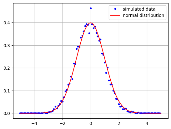
Because the phase shifts \(\phi_k\) are randomly and uniformly distributed, the variables \(x\) and \(y\) are sums of identically distributed cosine and sine terms respectively. The Central Limit Theorem of statistics then says that \(x\) and \(y\) will have a normal distribution with zero mean and variance \(\sigma^2 =n/2\) in the limit of large number \(n\) of scatterers. We can verify this with a simple piece of code in which we set \(n=10000\):
def X(n):
    return np.sum(np.cos(4*np.pi*(np.random.rand(n)-0.5)))/np.sqrt(n/2)

n= 10000
Xs = [X(n) for i in range(10000)]
y, x = np.histogram(Xs, 100, range=[-5,5])
plt.plot(x[:-1], y/1000, 'b.', label='simulated data')
plt.plot(x, norm.pdf(x), '-r', label='normal distribution')
plt.grid()
plt.legend()
plt.show()
Furthermore, \(x\) and \(y\) are uncorrelated since, in the expression for covariance of \(x\) and \(y\), the sums of products of cosine and sine terms cancel to zero. This means that \(x + {\bf i}y\), and hence the observed single look complex signal \(S_{vv}\) (see Eq. (1.8)), has a complex normal distribution .
Now what about the pixels values in the Sentinel-1 VV intensity images? They are given by the square of the amplitude of \(S_{vv}\),
(Actually averages of the above, as we'll see later.) We can write this in the form
where
is the sum of the squares of two variables with independent standard normal distributions. Applying the
- Theorem: If the measurements \(x_i,\ i=1\dots m\), are independent and standard normally distributed (i.e., with mean \(0\) and variance \(1\)), then the variable \(x=\sum_{i=1}^m x_i^2\) is chi-square distributed with \(m\) degrees of freedom, given by
we see that \(u\) is chi-square distributed with degrees of freedom \(m=2\),
since \(\Gamma(1)=1\).
To simplify the notation, let \(s=|S_{vv}|^2 \) and \(a=|S^a_{vv}|^2\). Then from (1.10)
To get the distribution \(p_s(s)\) of the observed signal from the distribution of \(u\), we apply the standard transformation formula
Compare this with the definition of the exponential probability distribution
We conclude that the measured intensity signal \(s=|S_{vv}|^2\) has an exponential distribution with mean and variance equal to the underlying signal strength \(a=|S^a_{vv}|^2\).
So far so good, however we still haven't quite characterized the statistics of the pixels in the intensity bands of the Sentinel-1 images.
Multi-look SAR statistics
Multi-look processing essentially corresponds to the averaging of neighborhood pixels with the objective of reducing speckle and compressing the data. In practice, the averaging is often not performed in the spatial domain, but rather in the frequency domain during range/azimuth compression of the received signal.
Look averaging takes place at the cost of spatial resolution. The spatial resolution attainable with SAR satellite platforms involves, among many other considerations, a compromise between azimuthal resolution and swath width, see Moreira et al. (2013) for a good discussion. In the Sentinel-1 Interferometric Wide Swath acquisition mode, the pixels are about 20m \(\times\) 4m (azimuth \(\times\) range) in extent and the swath widths are about 250km. For the multi-looking procedure, five cells are incoherently averaged in the range direction to achieve approx. \(20m \times 20m\) resolution. The pixels are then resampled to \(10\times 10\ m^2\). (Note that spatial resolution is a measure of the system's ability to distinguish between adjacent targets while pixel spacing is the distance between adjacent pixels in an image, measured in metres.) The look averaging process, which we can symbolize using angular brackets as \(\langle |S_{vv}|^2 \rangle\) or \(\langle |S_{vh}|^2 \rangle\), has the desirable effect of reducing speckle (at the cost of resolution) in the intensity images. We can see this as follows, first quoting another well-known Theorem in statistics:
- Theorem: If the quantities \(s_i,\ i=1\dots m,\) are independent and each have exponential distributions given by Eq. (1.16), then \(x = \sum_{i=1}^m s_i\) has the gamma distribution Eq. (1.1) with \(\alpha=m,\ \beta=a\). Its mean is \(\alpha\beta =ma\) and its variance is \(\alpha\beta^2 = ma^2.\)
Again with the notation \(s=|S_{vv}|^2 \) and \(a=|S^a_{vv}|^2\), if intensity measurements \(s\) are summed over \(m\) looks to give \(\sum_{i=1}^m s_i\), then according to this Theorem the sum (not the average!) will be gamma distributed with \(\alpha= m\) and \(\beta=a\), provided the \(s_i\) are independent. The look-averaged image is
and its mean value is
Now we see that the histogram of the Sentinel-1 multi-look image \(\langle s\rangle =\langle |S_{vv}|^2 \rangle\) follows a gamma distribution with the parameters
as we demonstrated earlier with the measured histogram.
The covariance representation of the dual pol multilook images is
Equivalent number of looks
The variance of \(\langle s\rangle\) is given by
where we have used the fact that the variance of the gamma distribution is \(\alpha\beta'^2=ma^2\). Thus the variance of the look-averaged image, the speckle effect, decreases inversely with the number of looks.
In practice, the neighborhood pixel intensities contributing to the look average will not be completely independent, but correlated to some extent. This is accounted for by defining an equivalent number of looks (ENL) whose definition is motivated by Eq. (1.21), that is,
In general it will be smaller than \(m\). Let's see what we get for our subset of the airport image:
mean ** 2 / variance
4.324058395540761
The value given by the provider (ESA) for the IW mode imagery in the GEE archive is ENL = 4.4, an average over all swaths, so our spatial subset seems to be fairly representative.
Outlook
Now we have a good idea of the statistics of the Sentinel-1 images on the GEE. In Part 2 of the Tutorial we will discuss statistical methods to detect changes in two Sentinel-1 images acquired at different times.