Page Summary
-
This tutorial introduces the Multivariate Alteration Detection (MAD) transformation and its iteratively re-weighted version (iMAD) for detecting changes in satellite imagery using Google Earth Engine (GEE).
-
The MAD transformation creates difference images (MAD variates) from two multi-band images by maximizing the correlation between linear combinations of their bands.
-
The MAD variates are mutually uncorrelated, and their variances indicate the magnitude of change, with the first variate showing the minimum variance and subsequent ones showing minimum variance subject to being uncorrelated with previous ones.
 View source on GitHub
Context
With the great tools available in Google Earth Engine (GEE) it is easy to generate satellite image differences and time series animations which visualize changes on the Earth surface, sometimes quite dramatically. Such representations are very good as eye-openers to give a conceptual, overall impression of change. They may, however, be perceived differently from person to person and not allow more than subjective interpretation. With more objective and rigorous statistical methods one can often extract more and better change information on both pixel and patch/field levels.
The Multivariate Alteration Detection (MAD) transformation was proposed and developed some time ago by Allan Nielsen and his coworkers at the Technical University of Denmark and later extended to an iteratively re-weighted version called IR-MAD or iMAD. The iMAD algorithm has since found widespread application for the generation of change information from visual/infrared imagery as well as for performing relative radiometric normalization of image pairs.
This tutorial is intended to familiarize GEE users with the iMAD method so that they may use it with confidence in their research wherever they think it might be appropriate. It is based on material taken from Chapter 9 of Canty (2019). In preparing the tutorial we have tried to take as much advantage as possible of the GEE platform to illustrate and demonstrate the theory interactively.
Outline
The tutorial is split into three parts, of which this is the first:
1. The MAD Transformation
2. The iMAD Algorithm
3. Radiometric Normalization and Harmonization
In Part 3, a convenient Jupyter widget interface for running the iMAD algorithm from a Docker container is also described.
Prerequisites
Little prior knowledge is required to follow the discussion, apart from some familiarity with the GEE API and a basic, intuitive understanding of the simple statistical concepts of probability distributions and their moments, in particular, mean, variance (var) and covariance (cov). Since we'll be working with multispectral imagery, in the course of the tutorial we'll frequently mention the so-called dispersion matrix or variance-covariance matrix, or simply covariance matrix for short. The covariance matrix of a set of measured variables \(X_i,\ i=1\dots N\), such as the band-wise values of a multispectral image pixel, is defined as
where
Here, \(\bar X_i\) denotes mean value and \(\langle\dots\rangle\) is ensemble average. The covariance matrix is symmetric about its principal diagonal. The correlation between \(X_i\) and \(X_j\) is defined as the normalized covariance
Since we are in a Colab environment we will use the Python API, but it is so similar to the JavaScript version that this should pose no problems to anyone not acquainted with it.
Preliminaries
The cells below execute the necessary formalities for accessing Earth Engine from this Colab notebook. They also import the various Python add-ons needed, including the geemap interactive map package, and define a few helper routines for displaying results.
import ee

ee.Authenticate(auth_mode='notebook')
ee.Initialize()
# Import other packages used in the tutorial
%matplotlib inline
import geemap
import numpy as np
import random, time
import matplotlib.pyplot as plt
from scipy.stats import norm, chi2

from pprint import pprint  # for pretty printing
# Truncate a 1-D array to dec decimal places
def trunc(values, dec = 3):
    return np.trunc(values*10**dec)/(10**dec)
# Display an image in a one percent linear stretch
def display_ls(image, map, name, centered = False):
    bns = image.bandNames().length().getInfo()
    if bns == 3:
        image = image.rename('B1', 'B2', 'B3')
        pb_99 = ['B1_p99', 'B2_p99', 'B3_p99']
        pb_1 = ['B1_p1', 'B2_p1', 'B3_p1']
        img = ee.Image.rgb(image.select('B1'), image.select('B2'), image.select('B3'))
    else:
        image = image.rename('B1')
        pb_99 = ['B1_p99']
        pb_1 = ['B1_p1']
        img = image.select('B1')
    percentiles = image.reduceRegion(ee.Reducer.percentile([1, 99]), maxPixels=1e11)
    mx = percentiles.values(pb_99)
    if centered:
        mn = ee.Array(mx).multiply(-1).toList()
    else:
        mn = percentiles.values(pb_1)
    map.addLayer(img, {'min': mn, 'max': mx}, name)
Simple Differences
Let's begin by considering two \(N\)-band optical/infrared images of the same scene acquired with the same sensor at two different times, between which ground reflectance changes have occurred at some locations but not everywhere. To see those changes we can "flick back and forth" between gray scale or RGB representations of the images on a computer display. Alternatively we can simply subtract one image from the other and, provided the intensities at the two time points have been calibrated or normalized in some way, examine the difference. Symbolically the difference image is
where
are 'typical' pixel vectors (more formally: random vectors) representing the first and second image, respectively.
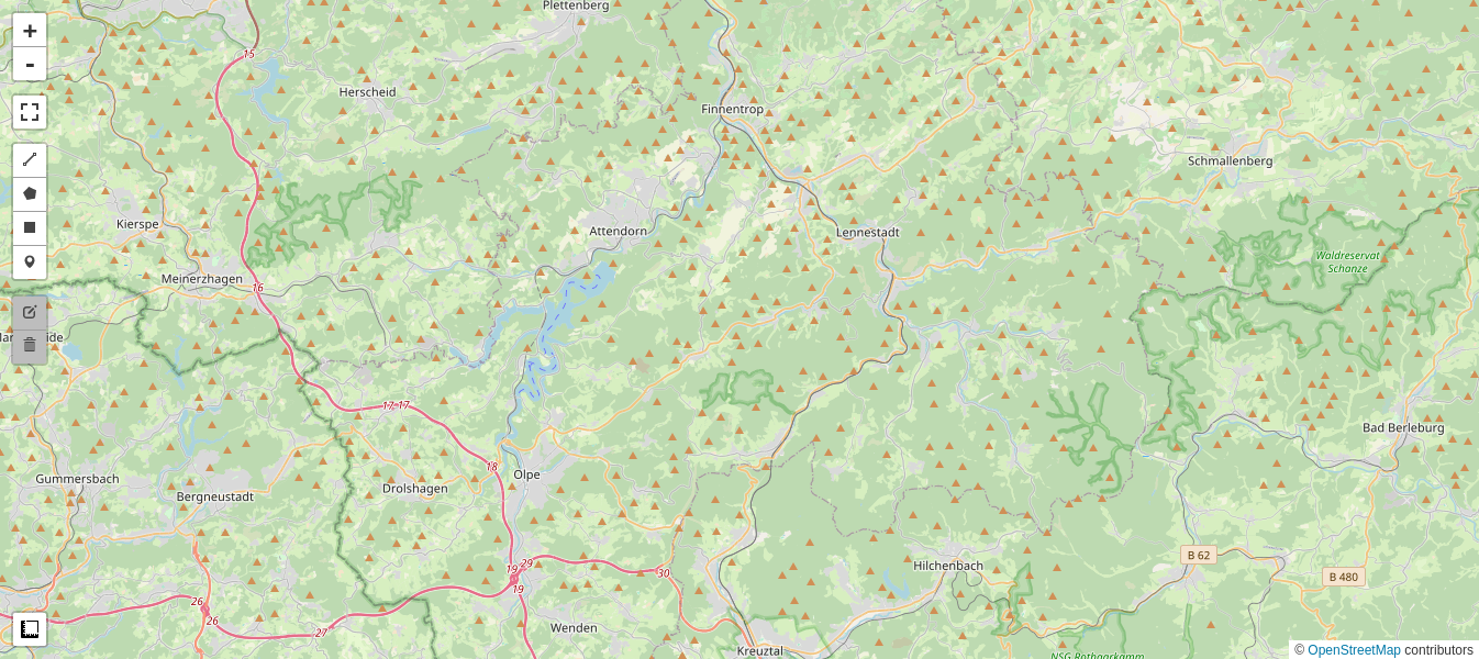
Landkreis Olpe
For example, here is an area of interest (aoi) covering a heavily forested administrative district (Landkreis Olpe) in North Rhine Westphalia, Germany. Due to severe drought in recent years large swaths of shallow-root coniferous trees have died and been cleared away, leaving deciduous trees for the most part untouched.
aoi = ee.FeatureCollection(
    'projects/google/imad_tutorial/landkreis_olpe_aoi').geometry()
We first collect two Sentinel-2 scenes which bracket some of the recent clear cutting (June, 2021 and June, 2022) and print out their timestamps. For demonstration purposes we choose top of atmosphere reflectance since the MAD transformation does not require absolute surface reflectances.
def collect(aoi, t1a ,t1b, t2a, t2b):
    try:
        im1 = ee.Image( ee.ImageCollection("COPERNICUS/S2_HARMONIZED")
                               .filterBounds(aoi)
                               .filterDate(ee.Date(t1a), ee.Date(t1b))
                               .filter(ee.Filter.contains(rightValue=aoi,leftField='.geo'))
                               .sort('CLOUDY_PIXEL_PERCENTAGE')
                               .first()
                               .clip(aoi) )
        im2 = ee.Image( ee.ImageCollection("COPERNICUS/S2_HARMONIZED")
                               .filterBounds(aoi)
                               .filterDate(ee.Date(t2a), ee.Date(t2b))
                               .filter(ee.Filter.contains(rightValue=aoi,leftField='.geo'))
                               .sort('CLOUDY_PIXEL_PERCENTAGE')
                               .first()
                               .clip(aoi) )
        timestamp = im1.date().format('E MMM dd HH:mm:ss YYYY')
        print(timestamp.getInfo())
        timestamp = im2.date().format('E MMM dd HH:mm:ss YYYY')
        print(timestamp.getInfo())
        return (im1, im2)
    except Exception as e:
        print('Error: %s'%e)

im1, im2 = collect(aoi, '2021-06-01', '2021-06-30', '2022-06-01', '2022-06-30')
Sun Jun 13 10:36:49 2021
Thu Jun 16 10:46:56 2022
In order to view the images, we instantiate an interactive map located at the center of the aoi. Since the map requires lat/long coordinates we have to reverse the long/lat order returned from the coordinates() method of the ee.Geometry.centroid() object:
# Interactive map
M1 = geemap.Map()
M1.centerObject(aoi, 11)

M1
Then we display RGB composites of the first 3 (visual) bands of the Sentinel images as well as their difference. We use the previously defined function display_ls() to display the images in a one percent linear stretch.
visirbands = ['B2','B3','B4','B8','B11','B12']
visbands = ['B2','B3','B4']

diff = im1.subtract(im2).select(visbands)
display_ls(im1.select(visbands), M1, 'Image 1')
display_ls(im2.select(visbands), M1, 'Image 2')
display_ls(diff, M1, 'Difference')
Small intensity differences (the gray-ish background in the difference image above) indicate no change, large positive (bright) or negative (dark) colors indicate change. The most obvious changes are in fact due to the clear cutting. Decision thresholds can be set to define significant changes. The thresholds are usually expressed in terms of standard deviations from the mean difference value, which is taken to correspond to no change. The per-band variances of the difference images are simply
or, if the bands are uncorrelated, about twice as noisy as the individual image bands. Normally \(X_i\) and \(Y_i\) are positively correlated (\({\rm cov}(X_i,Y_i) > 0\)) so the variance of \(Z_i\) is somewhat smaller. When the difference signatures in the spectral channels are combined so as to try to characterize the nature of the changes that have taken place, one speaks of spectral change vector analysis.
While the recent clear cuts are fairly easily identified as (some but not all of) the dark areas in the simple difference image above, it is possible to derive a better and more informative change map. This involves taking greater advantage of the statistical properties of the images.
The MAD Transformation
Let's make a linear combination of the intensities for all \(N\) bands in the first image \(X\), thus creating a scalar image
The symbol \({\bf a}^\top\) denotes the transpose of the column vector \({\bf a}=\begin{pmatrix}a_1\cr a_2\cr\vdots\cr a_N\end{pmatrix}\), in other words the row vector \({\bf a}^\top = (a_1,a_2 \dots a_N)\).
The expression \({\bf a}^\top X\) is called an inner vector product. The vector of coefficients \({\bf a}\) is as yet unspecified. We'll do the same for the second image \(Y\), forming the linear combination
and then look at the scalar difference \(U-V\). Change information is now contained, for the time being, in a single image rather than distributed among all \(N\) bands.
We have of course to choose the coefficient vectors \({\bf a}\) and \({\bf b}\) in some suitable way. In Nielsen et al. (1998) it is suggested that they be determined by making the transformed images \(U\) and \(V\) as similar as they can be before taking their difference. This sounds at first counter-intuitive: Why make the images similar when we want to see the dissimilarities? The crux is that, in making them match one another by taking suitable linear combinations, we ensure that pixels in the transformed images \(U\) and \(V\) at which indeed no change has taken place will be as similar as possible before they are compared (subtracted). The genuine changes will then, it is hoped, be all the more apparent in the difference image.
This process of "similar making" can be accomplished in statistics with standard Canonical Correlation Analysis (CCA), a technique first described by Harold Hotelling in 1936. Canonical Correlation Analysis of the images represented by Equations (1) and (2) maximizes the correlation
between the random variables \(U\) and \(V\), which is just what we want.
One technical point: Arbitrary multiples of \(U\) and \(V\) would clearly have the same correlation (the multiples will cancel off in numerator and denominator), so a constraint must be chosen. A convenient one is
For those more versed in linear algebra the details of CCA are given in Canty (2019) beginning on page 385. It all boils down to solving two so-called generalized eigenvalue problems for determining the transformation vectors \({\bf a}\) and \({\bf b}\) in Equations (1) and (2), respectively. There is not just one solution but rather \(N\) solutions. They consist of the \(N\) pairs of eigenvectors \(({\bf a}^i, {\bf b}^i)\),
and, correspondingly, the \(N\) pairs of canonical variates \((U_i, V_i),\ i= 1\dots N\). (Readers familiar with Principal Components Analysis (PCA) will recognize the similarity. When applying PCA to an N-band image, an ordinary (rather than a generalized) eigenvalue problem is solved to maximize variance, resulting in \(N\) principal component bands.)
Unlike the bands of the original images \(X\) and \(Y\), which are ordered by spectral wavelength, the canonical variates are ordered by similarity or correlation. The difference images
contain the change information and are called the MAD variates.
Auxiliary functions
To run the MAD transformation on GEE image pairs we need some helper routines. These are coded below. The first, called covarw(), returns the weighted covariance matrix of an \(N\)-band image as well as a weighted, centered (mean-zero) version of the image. Why it is important to weight the pixels before centering or calculating the covariance matrix will become apparent in Part 2 of the tutorial.
def covarw(image, weights = None, scale = 20, maxPixels = 1e10):
    '''Return the weighted centered image and its weighted covariance matrix'''
    try:
        geometry = image.geometry()
        bandNames = image.bandNames()
        N = bandNames.length()
        if weights is None:
            weights = image.constant(1)
        weightsImage = image.multiply(ee.Image.constant(0)).add(weights)
        means = image.addBands(weightsImage) \
                    .reduceRegion(ee.Reducer.mean().repeat(N).splitWeights(),
                                scale = scale,
                                maxPixels = maxPixels) \
                    .toArray() \
                    .project([1])
        centered = image.toArray().subtract(means)
        B1 = centered.bandNames().get(0)
        b1 = weights.bandNames().get(0)
        nPixels = ee.Number(centered.reduceRegion(ee.Reducer.count(),
                                                scale = scale,
                                                maxPixels = maxPixels).get(B1))
        sumWeights = ee.Number(weights.reduceRegion(ee.Reducer.sum(),
                                                    geometry = geometry,
                                                    scale = scale,
                                                    maxPixels = maxPixels).get(b1))
        covw = centered.multiply(weights.sqrt()) \
                    .toArray() \
                    .reduceRegion(ee.Reducer.centeredCovariance(),
                                    geometry = geometry,
                                    scale = scale,
                                    maxPixels = maxPixels) \
                    .get('array')
        covw = ee.Array(covw).multiply(nPixels).divide(sumWeights)
        return (centered.arrayFlatten([bandNames]), covw)
    except Exception as e:
        print('Error: %s'%e)
The second routine, called corr(), transforms a covariance matrix to the equivalent correlation matrix by dividing by the square roots of the variances, see Equation (3).
def corr(cov):
    '''Transform covariance matrix to correlation matrix'''
    # diagonal matrix of inverse sigmas
    sInv = cov.matrixDiagonal().sqrt().matrixToDiag().matrixInverse()
    # transform
    corr = sInv.matrixMultiply(cov).matrixMultiply(sInv).getInfo()
    # truncate
    return [list(map(trunc, corr[i])) for i in range(len(corr))]
For example the code below calculates the (unweighted) covariance matrix of the visual and infrared bands of the image im1 and prints out the corresponding correlation matrix.
_, cov = covarw(im1.select(visirbands))
pprint(corr(cov))
[[np.float64(0.999),
  np.float64(0.952),
  np.float64(0.949),
  np.float64(0.063),
  np.float64(0.647),
  np.float64(0.79)],
 [np.float64(0.952),
  np.float64(1.0),
  np.float64(0.927),
  np.float64(0.292),
  np.float64(0.772),
  np.float64(0.847)],
 [np.float64(0.949),
  np.float64(0.927),
  np.float64(1.0),
  np.float64(0.008),
  np.float64(0.741),
  np.float64(0.893)],
 [np.float64(0.063),
  np.float64(0.292),
  np.float64(0.008),
  np.float64(1.0),
  np.float64(0.486),
  np.float64(0.22)],
 [np.float64(0.647),
  np.float64(0.772),
  np.float64(0.741),
  np.float64(0.486),
  np.float64(1.0),
  np.float64(0.933)],
 [np.float64(0.79),
  np.float64(0.847),
  np.float64(0.893),
  np.float64(0.22),
  np.float64(0.933),
  np.float64(0.999)]]
Note that the spectral bands of the image are generally highly and positively correlated with one another.
By stacking the images one atop the other we can use the helper functions to display the between image correlations
They can be found in the diagonal of the upper left \(6\times 6\) submatrix of the correlation matrix for the stacked image.
im12 = im1.select(visirbands).addBands(im2.select(visirbands))
_, covar = covarw(im12)
correl = np.array(corr(covar))
print(np.diag(correl[:6, 6:]))
[0.799 0.784 0.683 0.867 0.666 0.632]
It is these between image correlations that the MAD algorithm tries to maximize.
The third and last auxiliary routine, geneiv(), is the core of CCA and the MAD transformation. It solves the generalized eigenproblem,
for two \(N\times N\) matrices \(C\) and \(B\), returning the \(N\) solutions, or eigenvectors, \(X_i\) and the \(N\) eigenvalues \(\lambda_i, \ i=1\dots N\).
def geneiv(C,B):
    '''Return the eigenvalues and eigenvectors of the generalized eigenproblem
                         C*X = lambda*B*X'''
    try:
        C = ee.Array(C)
        B = ee.Array(B)
        #  Li = choldc(B)^-1
        Li = ee.Array(B.matrixCholeskyDecomposition().get('L')).matrixInverse()
        #  solve symmetric, ordinary eigenproblem Li*C*Li^T*x = lambda*x
        Xa = Li.matrixMultiply(C) \
            .matrixMultiply(Li.matrixTranspose()) \
            .eigen()
        #  eigenvalues as a row vector
        lambdas = Xa.slice(1, 0, 1).matrixTranspose()
        #  eigenvectors as columns
        X = Xa.slice(1, 1).matrixTranspose()
        #  generalized eigenvectors as columns, Li^T*X
        eigenvecs = Li.matrixTranspose().matrixMultiply(X)
        return (lambdas, eigenvecs)
    except Exception as e:
        print('Error: %s'%e)
The next cell codes the MAD transformation itself in the function mad_run(), taking as input two multiband images and returning the canonical variates
the MAD variates
as well as the sum of the squares of the standardized MAD variates,
The MAD transformation
def mad_run(image1, image2, scale = 20):
    '''The MAD transformation of two multiband images'''
    try:
        image = image1.addBands(image2)
        region = image.geometry()
        nBands = image.bandNames().length().divide(2)
        centeredImage,covarArray = covarw(image,scale=scale)
        bNames = centeredImage.bandNames()
        bNames1 = bNames.slice(0,nBands)
        bNames2 = bNames.slice(nBands)
        centeredImage1 = centeredImage.select(bNames1)
        centeredImage2 = centeredImage.select(bNames2)
        s11 = covarArray.slice(0,0,nBands).slice(1,0,nBands)
        s22 = covarArray.slice(0,nBands).slice(1,nBands)
        s12 = covarArray.slice(0,0,nBands).slice(1,nBands)
        s21 = covarArray.slice(0,nBands).slice(1,0,nBands)
        c1 = s12.matrixMultiply(s22.matrixInverse()).matrixMultiply(s21)
        b1 = s11
        c2 = s21.matrixMultiply(s11.matrixInverse()).matrixMultiply(s12)
        b2 = s22
        # solution of generalized eigenproblems
        lambdas, A = geneiv(c1,b1)
        _,       B = geneiv(c2,b2)
        rhos = lambdas.sqrt().project(ee.List([1]))
        # MAD variances
        sigma2s = rhos.subtract(1).multiply(-2).toList()
        sigma2s = ee.Image.constant(sigma2s)
        # ensure sum of correlations between X and U is positive
        tmp = s11.matrixDiagonal().sqrt()
        ones = tmp.multiply(0).add(1)
        tmp = ones.divide(tmp).matrixToDiag()
        s = tmp.matrixMultiply(s11).matrixMultiply(A).reduce(ee.Reducer.sum(),[0]).transpose()
        A = A.matrixMultiply(s.divide(s.abs()).matrixToDiag())
        # ensure positive correlation between U and V
        tmp = A.transpose().matrixMultiply(s12).matrixMultiply(B).matrixDiagonal()
        tmp = tmp.divide(tmp.abs()).matrixToDiag()
        B = B.matrixMultiply(tmp)
        # canonical and MAD variates
        centeredImage1Array = centeredImage1.toArray().toArray(1)
        centeredImage2Array = centeredImage2.toArray().toArray(1)
        U = ee.Image(A.transpose()).matrixMultiply(centeredImage1Array) \
                    .arrayProject([0]) \
                    .arrayFlatten([bNames2])
        V = ee.Image(B.transpose()).matrixMultiply(centeredImage2Array) \
                    .arrayProject([0]) \
                    .arrayFlatten([bNames2])
        MAD = U.subtract(V)
        #  chi square image
        Z = MAD.pow(2) \
                .divide(sigma2s) \
                .reduce(ee.Reducer.sum()) \
                .clip(region)
        return (U, V, MAD, Z)
    except Exception as e:
        print('Error: %s'%e)
After setting up the MAD transformation on the six visual and infrared bands of the Landkreis Olpe images,
U, V, MAD, Z = mad_run(im1.select(visirbands), im2.select(visirbands))
we display an RGB composite of the first 3 MAD variates, together with the original images and their simple difference:
M2 = geemap.Map()
M2.centerObject(aoi, 11)
display_ls(im1.select(visbands), M2, 'Image 1')
display_ls(im2.select(visbands), M2, 'Image 2')
display_ls(diff, M2, 'Difference')
display_ls(MAD.select(0, 1, 2), M2, 'MAD Image', True)

M2
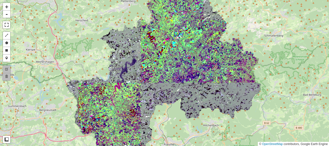
The richness in colors in the MAD image is a consequence of the decoupling (orthogonalization) of the MAD components, as will be explained below.
Pretty colors notwithstanding, when compared with the simple difference image the result is mittelprächtig (German slang for "not so hot"), and certainly no easier to interpret. However we're not finished.
The canonical variates have very nice properties indeed. They are all mutually uncorrelated except for the pairs \((U_i,V_i)\), and these are ordered by decreasing positive correlation:
with \(\rho_1 \ge \rho_2 \ge\dots \ge\rho_N\).
Stacking the images \(U\) and \(V\), these facts can be read from the \(12\times 12\) correlation matrix:
_, covar = covarw(U.addBands(V))
correl = np.array(corr(covar))
pprint(correl)
print('rho =', np.diag(correl[:6,6:]))
array([[ 1.   ,  0.001, -0.   ,  0.   , -0.   ,  0.   ,  0.924,  0.   ,
        -0.   ,  0.   , -0.   , -0.   ],
       [ 0.001,  1.   ,  0.   ,  0.   , -0.   , -0.   ,  0.   ,  0.864,
         0.   ,  0.   , -0.   , -0.   ],
       [-0.   ,  0.   ,  1.   ,  0.   ,  0.   , -0.   , -0.   ,  0.   ,
         0.708, -0.   ,  0.   , -0.   ],
       [ 0.   ,  0.   ,  0.   ,  0.999,  0.   ,  0.   ,  0.   ,  0.   ,
        -0.   ,  0.642,  0.   ,  0.   ],
       [-0.   , -0.   ,  0.   ,  0.   ,  1.   ,  0.   , -0.   , -0.   ,
         0.   ,  0.   ,  0.536,  0.   ],
       [ 0.   , -0.   , -0.   ,  0.   ,  0.   ,  1.   , -0.   , -0.   ,
        -0.   ,  0.   ,  0.   ,  0.369],
       [ 0.924,  0.   , -0.   ,  0.   , -0.   , -0.   ,  0.999,  0.   ,
        -0.   ,  0.   , -0.   , -0.   ],
       [ 0.   ,  0.864,  0.   ,  0.   , -0.   , -0.   ,  0.   ,  0.999,
         0.   ,  0.   , -0.   , -0.   ],
       [-0.   ,  0.   ,  0.708, -0.   ,  0.   , -0.   , -0.   ,  0.   ,
         0.999, -0.   ,  0.   , -0.   ],
       [ 0.   ,  0.   , -0.   ,  0.642,  0.   ,  0.   ,  0.   ,  0.   ,
        -0.   ,  1.   ,  0.   ,  0.   ],
       [-0.   , -0.   ,  0.   ,  0.   ,  0.536,  0.   , -0.   , -0.   ,
         0.   ,  0.   ,  1.   ,  0.   ],
       [-0.   , -0.   , -0.   ,  0.   ,  0.   ,  0.369, -0.   , -0.   ,
        -0.   ,  0.   ,  0.   ,  0.999]])
rho = [0.924 0.864 0.708 0.642 0.536 0.369]
The MAD variates themselves are consequently also mutually uncorrelated, their covariances being given by
and their variances by
where the last equality follows from the constraint Equation (4). Let's check.
# display MAD covariance matrix
_, covar = covarw(MAD)
covar = covar.getInfo()
[list(map(trunc,covar[i])) for i in range(len(covar))]
[[np.float64(0.078),
  np.float64(0.0),
  np.float64(-0.0),
  np.float64(0.0),
  np.float64(0.0),
  np.float64(0.0)],
 [np.float64(0.0),
  np.float64(0.14),
  np.float64(0.0),
  np.float64(-0.0),
  np.float64(-0.0),
  np.float64(0.0)],
 [np.float64(-0.0),
  np.float64(0.0),
  np.float64(0.303),
  np.float64(0.0),
  np.float64(-0.0),
  np.float64(-0.0)],
 [np.float64(0.0),
  np.float64(-0.0),
  np.float64(0.0),
  np.float64(0.372),
  np.float64(0.0),
  np.float64(0.0)],
 [np.float64(0.0),
  np.float64(-0.0),
  np.float64(-0.0),
  np.float64(0.0),
  np.float64(0.482),
  np.float64(0.0)],
 [np.float64(0.0),
  np.float64(0.0),
  np.float64(-0.0),
  np.float64(0.0),
  np.float64(0.0),
  np.float64(0.656)]]
The first MAD variate has minimum variance in its pixel intensities. The second MAD variate has minimum variance subject to the condition that its pixel intensities are statistically uncorrelated with those in the first variate; the third has minimum spread subject to being uncorrelated with the first two, and so on. Depending on the type of change present, any of the components may exhibit significant change information, although it tends to be concentrated in the first few MAD variates. One of the nicest aspects of the MAD transformation is that it can sort different categories of change into different, uncorrelated image bands.
However, the result, as we saw, needs some improvement. This is the subject of Part 2.