HISTARFM - How to Work with Gap-Filled Imagery

Author(s): EIzquierdo

Overview

Although there is an extensive array of optical remote sensing sensors from a variety of satellites providing long time data records, their data are incapable of retrieving reliable land surface information when clouds, aerosols, shadows, and strong angular effects are present in the scenes. The mitigation of noise and gap filling of satellite data are preliminary and almost mandatory tasks for any remote sensing application aimed at effectively analyzing the earth's surface continuously through time.

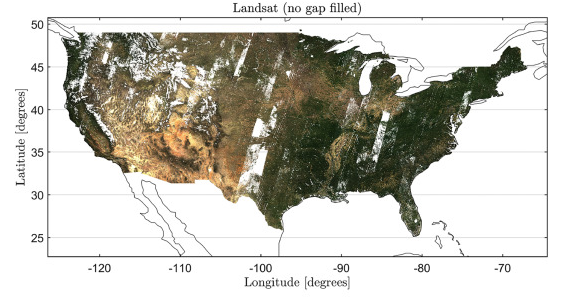
An example of cloud contaminated Landsat surface reflectance data

In 2020, to tackle this challenging problem Moreno-Martinez et al. (2020) proposed using the Google Earth Engine (GEE) cloud computing platform to implement the HIghly Scalable Temporal Adaptive Reflectance Fusion Model (HISTARFM). This method generates reduced noise and gap-free estimates of Landsat reflectance values at vast scales. Despite the computational power of GEE and the optimizations of HISTARFM, the computational burden and memory costs of HISTARFM are too high to carry out any extra computations after the gap-filling process. Therefore, the data have to be pre-processed in different study areas. We have generated data for number of world regions already, and in this tutorial we will show how to use it and provide examples of how you can improve your research and applications with this enhanced Landsat-based dataset.

Background

The HISTARFM database is a gap-filled monthly reflectance temporal series at 30m spatial resolution generated by the fusion of Landsat and Moderate Resolution Imaging Spectroradiometer (MODIS) temporal series. The fusion algorithm relies on a bias-aware Bayesian data assimilation scheme implemented in GEE. The approach uses two linked estimators operating synergistically to filter out random noise and reduce the bias of Landsat spectral reflectances. The first estimator is an optimal interpolator that produces Landsat reflectance estimation values by combining Landsat historical data, pre-computed from the available Landsat record, and fused MODIS and Landsat reflectances obtained from overpasses closest to the time of interest. The fusion of reflectances results from using an efficient pixel-wise linear regression model. The second linked estimator is a Kalman filter that corrects the bias of the reflectance produced by the first estimator. For more information about HISTARFM algorithm, see the Moreno-Martinez et al. 2020 manuscript.

Versions

HISTARFM has been updated and improved since its publication in 2020. At the present, there are two versions available:

Version 2 corresponds with the exact algorithm published in the original paper in 2020. It relies on the USGS Landsat collection 1 surface reflectance data.
Version 5 (the last available version) contains numerous updates and enhancements, such as:
- The new USGS Landsat collection 2 is used.
- A linear interpolation method has been included for the original Landsat bands with adaptive uncertainties depending on the interpolation temporal distance.
- The Aerosol Optical Depth and Atmospheric Opacities data layers are used for better cloud masking and to prevent cirrus clouds contamination.

Version 2 datasets will be updated to Version 5 in the future, but it will take time.

To access the databases, ask any questions and stay updated on the latest information and upcoming data, please join the following google group: histarfm-collection@googlegroups.com.

Study areas

HISTARFM contains two study areas so far, but the dataset is continuously being expanded in time and spatial coverage.

The CONUS database contains 154 images stored as assets. It corresponds with version 2, and temporal coverage ranges from 2009 to 2021. Each image in the ImageCollection covers the full CONUS, and each has the properties 'version', 'month', and 'year'. This information is also present in their file names. For example, the image called Gap_Filled_Landsat_CONUS_month_10_2009_v2 is an October 2009 image for the CONUS area. The CONUS database is available in this asset.
The European database is currently being generated with version 5 of the algorithm. It contains 8208 images from 2017 to 2020, and the study area is divided into tiles stored in the Google Cloud Platform as Cloud Optimized Geotiffs (COG). These COGs are provided as COG-backed Earth Engine assets in a publicly readable ImageCollection available here. In this case, the images have all the properties needed in their generation, but the name of the image only includes the month, year, study area, and the tile. As an example, the image called GF_2018_10_EUROPA_1 represents the image in October 2018 over the first tile in Europe.

Examples of use of the HISTARFM database

1. Importing and visualizing the database

a. Import the ImageCollection

In this tutorial, we focus on 2019 in the European continent. Using the code below, you will load the European HISTARFM database from 2017 to 2020. The ImageCollection is filtered in the desired year (e.g., 2019) using the ee function filter. After that, a function called EuropeanMosaic to map the image collection is defined to generate a mosaic image of the entire continent per month. The images in the new image collection will contain the properties: 'system:time_start', 'month', and 'year' from the original images. These properties will be necessary for the next steps of this tutorial. After that, a function called scaleError is defined to scale and mask the error bands and set 'DOY,' 'month', and 'year' properties in the images together with the 'system:time_start' of the original images.

// Import HISTARTFM database.
var GF_Landsat =
    ee.ImageCollection('projects/ee-emma/assets/GF_Landsat_Europe_C2');

// Filter per year.
var year = '2019';  // In version 5 the properties are in string format, it
                    // seems to be a limitation of adding properties to COGs In
                    // case of using version 2 data (CONUS), the metadata is in
                    // standard integer format: `var year = 2019;`

GF_Landsat = GF_Landsat.filter(ee.Filter.eq('year', year));

var months = GF_Landsat.aggregate_array('month').distinct().sort();
// Join all images of a month into a single image.
function EuropeanMosaic(num) {
  var ic = GF_Landsat.filter(ee.Filter.eq('month', num));
  var img = ic.mosaic().selfMask();
  return img.copyProperties(ic.first(), ['system:time_start', 'month', 'year']);
}
var GF_Landsat = ee.ImageCollection(months.map(EuropeanMosaic));
// Sort the ImageCollection considering the 'system:time_start' property.
GF_Landsat = GF_Landsat.sort('system:time_start');

// Scaling the data to reflectance units.
function scaleError(img) {
  var y = ee.Number.parse(img.get('year'));
  var m = ee.Number.parse(img.get('month'));
  var d = ee.Date.fromYMD(y, m, 15);
  var doy = d.getRelative('day', 'year').add(1);
  var scaled = img.select(['P.*']).multiply(0.5);
  return img.addBands(scaled, null, true)
      .set({'month': m, 'year': y, 'DOY': doy})
      .copyProperties(img, ['system:time_start']);
}

GF_Landsat = GF_Landsat.map(scaleError);

b. Visualization of HISTARFM data

Once the HISTARFM dataset is prepared, the RGB gap-filled Landsat reflectance mosaic filtered to a specific month and its first band error are displayed considering their visualization parameters.

// Set map options.
Map.setOptions('HYBRID');
Map.setCenter(14.76, 49.28, 4);

// Subset a single month for display (e.g. July, the 7th month).
var julyImg = GF_Landsat.filter(ee.Filter.eq('month', 7));

// Display the RGB gap-filled Landsat reflectance mosaic to the map.
var imageVisParam = {
  'opacity': 1,
  'bands': ['B3_mean_post', 'B2_mean_post', 'B1_mean_post'],
  'min': 0,
  'max': 2500,
  'gamma': 1
};
Map.addLayer(julyImg, imageVisParam, 'example July RGB');

// Display the error gap-filled Landsat reflectance mosaic to the map.
var imageVisParam =
    {'opacity': 1, 'bands': ['P1_postSD'], 'min': 0, 'max': 200, 'gamma': 1};
Map.addLayer(GF_Landsat, imageVisParam, 'example error B1');

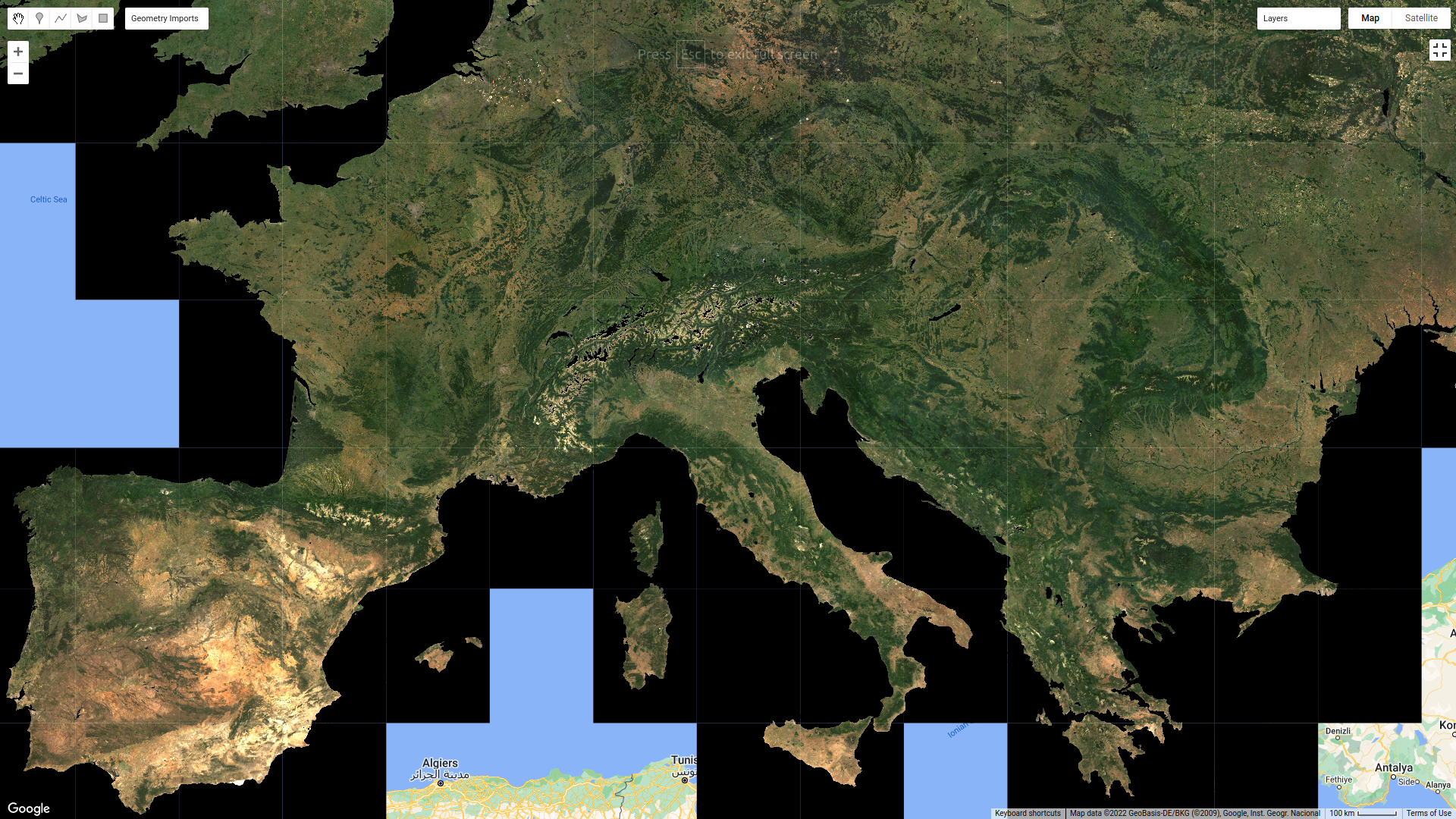
Example of a mosaic of the HISTARFM data over Europe for a given date

2. Calculate the timing and value of the maximum NDVI

The Normalized Difference Vegetation Index (NDVI) is the most widely used among the vast options of remotely sensed vegetation indices. The annual maximum value of NDVI is especially relevant in many studies as it represents the best status the vegetation can achieve in a growing season related to characteristics such as biomass, health, and photosynthetic capacity. To achieve this goal, the gap-free observations provided by the HISTARFM to correctly track vegetation phenology are very beneficial.

a. Calculate the NDVI and its error

The NDVI is based on the RED and NIR reflectances difference defined as follows:

$$ NDVI = \frac{NIR-RED}{NIR+RED} $$

As HISTARFM provides the reflectance values and reflectance uncertainties, it is possible to calculate the NDVI error using standard error propagation approach. Under the assumption of independence among the input variables, it is possible to obtain the error using a simplified approach:

$$ \epsilon(NDVI) = \frac{2}{(NIR+RED)^2} \cdot \sqrt{NIR^2 \cdot \epsilon(RED)^2 + RED^2 \cdot \epsilon(NIR)^2} $$

Reminder: NIR reflectance is the band called B4_mean_post and the RED is B3_mean_post in HISTARFM database.

Therefore, a function to calculate the NDVI and its error of the image collection is defined. The function ndvicompGF calculates NDVI and the error for each image. Additionally, the properties 'system:time_start', 'DOY', 'month', and 'year' are also included in the images from the original ones.

function ndvicompGF(img) {
  var ndvi =
      img.normalizedDifference(['B4_mean_post', 'B3_mean_post']).rename('NDVI');
  var errorNDVI = ee.Image().expression({
    expression: 'errorNDVI = 2 / pow(NIR + RED, 2) * ' +
        'sqrt(pow(NIR, 2) * pow(SD_RED, 2) + pow(RED, 2) * pow(SD_NIR, 2))',
    map: {
      RED: img.select('B3_mean_post'),
      NIR: img.select('B4_mean_post'),
      SD_RED: img.select('P3_postSD'),
      SD_NIR: img.select('P4_postSD')
    }
  });
  return img.addBands([ndvi, errorNDVI]).copyProperties(img, [
    'system:time_start', 'month', 'year', 'DOY'
  ]);
}

// Compute the NDVI and its error.
GF_Landsat = GF_Landsat.map(ndvicompGF);

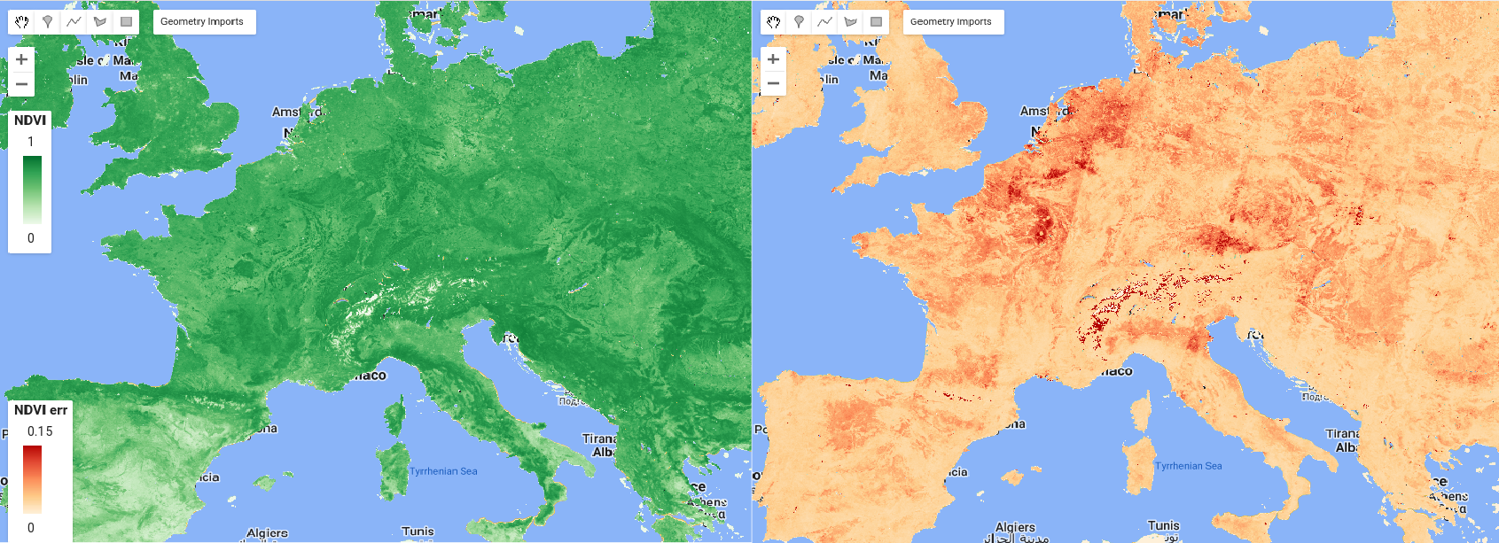
An example of the computed NDVI and its corresponding propagated error

b. Extracting growing season maximum NDVI value and timing

A function called maxMonth is defined to obtain the maximum NDVI value and the month when it is reached. Within this function, the GF_Landsat ImageCollection is mapped to add the month value as a band. Afterward, NDVI and Month bands are selected from the collection and reduced using a reducer ee.Reducer.max.

// Calculate the NDVI maximum value image.
function maxMonth(col) {
  col = col.map(function(img) {
    return img.addBands(
        ee.Image(ee.Number.parse(img.get('month'))).toByte().rename('Month'));
  });
  var theseBands = ['NDVI', 'Month'];
  return col.select(theseBands)
      .reduce(ee.Reducer.max(theseBands.length))
      .rename(theseBands);
}
var maxMonthNdvi = maxMonth(GF_Landsat);

c. Visualization of maximum NDVI value and the month

Once the variables are calculated, the NDVI maximum is displayed in whitenish (lower), greenish (medium) and blackish tones (higher values). The month is also displayed with a specific palette: bluenish tones for autumn and winter periods and greenish and reddish tones for spring and summer periods.

var imageVisParam = {
  'opacity': 1,
  'bands': ['NDVI'],
  'min': -1,
  'palette': ['ffffff', 'c5ff15', '94c00f', '617e0a', '000000']
};
Map.addLayer(maxMonthNdvi, imageVisParam, 'max NDVI');

var imageVisParam = {
  'opacity': 1,
  'bands': ['Month'],
  'min': 1,
  'max': 12,
  'palette': [
    '4306ff',  // January
    '4992ff',  // February
    'abe0ff',  // March
    'ccffd2',  // April
    '85ff89',  // May
    '34c045',  // Juny
    'ffd358',  // July
    'ff7321',  // August
    'ffa5a1',  // September
    'ceffe8',  // October
    '629fad',  // November
    '4d4d4d'   // December
  ]
};
Map.addLayer(maxMonthNdvi, imageVisParam, 'max month');

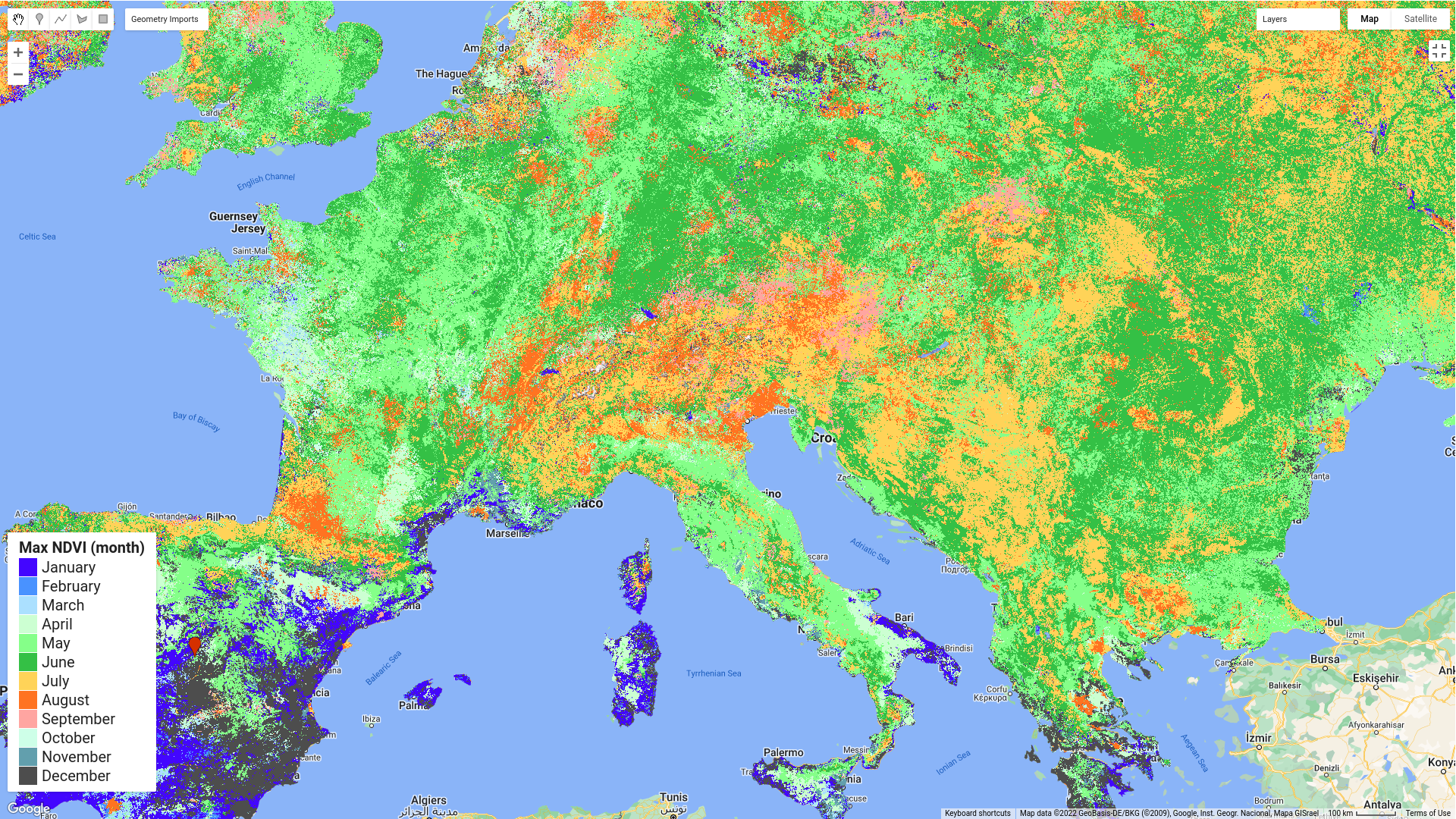
Timing of the maximum value of the NDVI for Europe (2019)

3. Temporal interpolation of the HISTARFM database

a. Creating a dummy ImageCollection with the desired temporal resolution

The first step to interpolating the HISTARFM database is the creation of a dummy (empty) ImageCollection with a regular time step sampling defined by tResolution. The function RegTimeColl requires a list of dates (interpreted as milliseconds since 1970-01-01T00:00:00Z) as input (timeRange in our example). Therefore, RegTimeColl creates the desired ImageCollection with the metadata ready ('DOY', 'system:time_start', and 'month'), which will be used to store the results of the interpolation.

// Desired interpolation temporal resolution in day units.
var tUnit = 'days';
var tResolution = 5;

// Create a list of DOYs.
var dateini = ee.Date(year + '-01-01');
var dateend = ee.Date(year + '-12-31');
var nSteps = dateend.difference(dateini, tUnit).divide(tResolution).floor();
var steps = ee.List.sequence(0, nSteps);
var timeRange = steps.map(function(i) {
  return dateini.advance(ee.Number(i).multiply(tResolution), tUnit).millis();
});

// Create a dummy collection with regular time space.
function RegTimeColl(date) {
  var DOY = ee.Date(date).getRelative('day', 'year').add(1);
  var m = ee.Number(ee.Date(date).get('month'));
  return ee.Image(DOY).rename('DOY').short().set(
      {'dummy': true, 'system:time_start': date, 'DOY': DOY, 'month': m});
}

var fiveDaysRes = ee.ImageCollection(timeRange.map(RegTimeColl));

b. HISTARFM linear interpolation

This section comprises two sub-steps: 1) Joining the ImageCollection created in the previous section called fiveDaysRes with the GF_Landsat ImageCollection from section 2.a, and 2) the interpolation step using the join from step 1.

b.1 Joining step

This step joins the fiveDaysRes ImageCollection with GF_Landsat ImageCollection. Each image in fiveDaysRes includes a property called LS where all the GF_Landsat images with a month of difference of fiveDaysRes are stored. The GF_Landsat selection is based on the 'system:time_start' property for both collections.

var join = ee.Join.saveAll('LS', 'system:time_start', true, null, true);
var nDays = 31;
var maxMilliDif = (nDays * 24 * 3600 * 1000);
var filter = ee.Filter.maxDifference(
    maxMilliDif, 'system:time_start', null, 'system:time_start');
var fiveDaysRes =
    ee.ImageCollection(join.apply(fiveDaysRes, GF_Landsat, filter));

b.2 Defining the interpolation function step

Once the fiveDaysRes ImageCollection contains the selected GF_Landsat images in the 'LS' property, an interpolation function (named CompositeInterpolate) is defined to map the fiveDaysRes ImageCollection. The interpolation between two points is a method to estimate new data between two known points. Considering $(x_0,y_0)$ and $(x_1,y_1)$ as these two known points, the linear prediction in an intermediate location is possible using the following equation:

$$ y = y_0 + \frac{y_1-y_0}{x_1-x_0} \cdot (x-x_0), $$

where $y_0$ and $y_1$ are the Gap-filled Landsat reflectances before and after respectively from GF_Landsat, $x_0$ and $x_1$ are their respective acquisition times (i.e. 'system:time_start'), $x$ is the time step for prediction, and $y$ is the predicted reflectance (of the new point) in the instant $x$.

Note two essential points:

Landsat images within the 'LS' property are sorted by 'system:time_start'. Therefore selecting the last element (i.e., get -1 element of the list) always is the after reflectance image, and selecting the previous to the last element (i.e., get -2 element of the list) always is the before reflectance image.
If the number of Landsat images in the 'LS' property is lower than 2 (extrapolation case), the image is either the first or the last in the fiveDaysRes ImageCollection. Therefore, the first or last images in fiveDaysRes are not interpolated. We only consider the values of Gap-filled Landsat reflectance contained in the 'LS' property.

// Get DOY of first and last day of the gap-filled reflectance ImageCollection.
var init_doy = ee.Image(GF_Landsat.first()).get('DOY');
var end_doy =
    ee.Image(GF_Landsat.sort('system:time_start', false).first()).get('DOY');

function CompositeInterpolate(img) {
  var list = ee.List(img.get('LS'));
  var LSbefore = ee.Image(
      ee.Algorithms.If(list.length().lt(2), list.get(0), list.get(-2)));
  var LSafter = ee.Image(
      ee.Algorithms.If(list.length().lt(2), list.get(0), list.get(-1)));
  var day = ee.Number(img.get('DOY'));
  var ini = ee.Number(LSbefore.get('DOY'));
  var end = ee.Number(LSafter.get('DOY'));
  var tdiff = end.subtract(ini);
  var slope = LSafter.subtract(LSbefore).divide(tdiff);
  var img_inter = slope.multiply(day.subtract(ini)).add(LSbefore);
  img_inter = img_inter.addBands(img_inter.select('P.*').int16(), null, true);
  img_inter = img_inter.where(
      day.lte(init_doy),
      GF_Landsat.filter(ee.Filter.eq('DOY', ee.Number(init_doy))).first());
  img_inter = img_inter.where(
      day.gte(end_doy),
      GF_Landsat.filter(ee.Filter.eq('DOY', ee.Number(end_doy))).first());
  var time = img.get('system:time_start');
  var month = img.get('month');
  return img_inter.set({
    'day': day,
    'month': month,
    'date_ini': ini,
    'date_end': end,
    'system:time_start': time,
    'year': year
  });
}

GF_Landsat = fiveDaysRes.map(CompositeInterpolate);

c. Visualization of the interpolated time series

In this case, a NDVI temporal series at one specific point is shown using a chart. Note that another band (i.e., reflectance or uncertainties) could also be visualized, only changing the selected band name in the code. We first define the ee.Geomatry.Point where the time series is going to be plotted. After that, the ui.Chart.image.series is used to visualize the NDVI temporarily upgraded temporal sequence. Finally, the chart is added to the map using the ee function Map.add.

// Define the geometry
var point = ee.Geometry.Point([-3.7010995437603, 40.41436099577093]);

// Define the chart
var chart = ui.Chart.image
                .series({
                  imageCollection: GF_Landsat.select('NDVI'),
                  region: point,
                  scale: 10,
                  reducer: ee.Reducer.first()
                })
                .setOptions({
                  title: ' NDVI',
                  vAxis: {title: 'NDVI'},
                  hAxis: {title: 'Time'},
                  series: {
                    0: {
                      color: '800000',
                      lineWidth: 2,
                      pointSize: 4,
                      curveType: 'function'
                    }
                  }
                });

// Add the chart to the map.
chart.style().set({position: 'top-left', width: '300px', height: '200px'});
Map.add(chart);

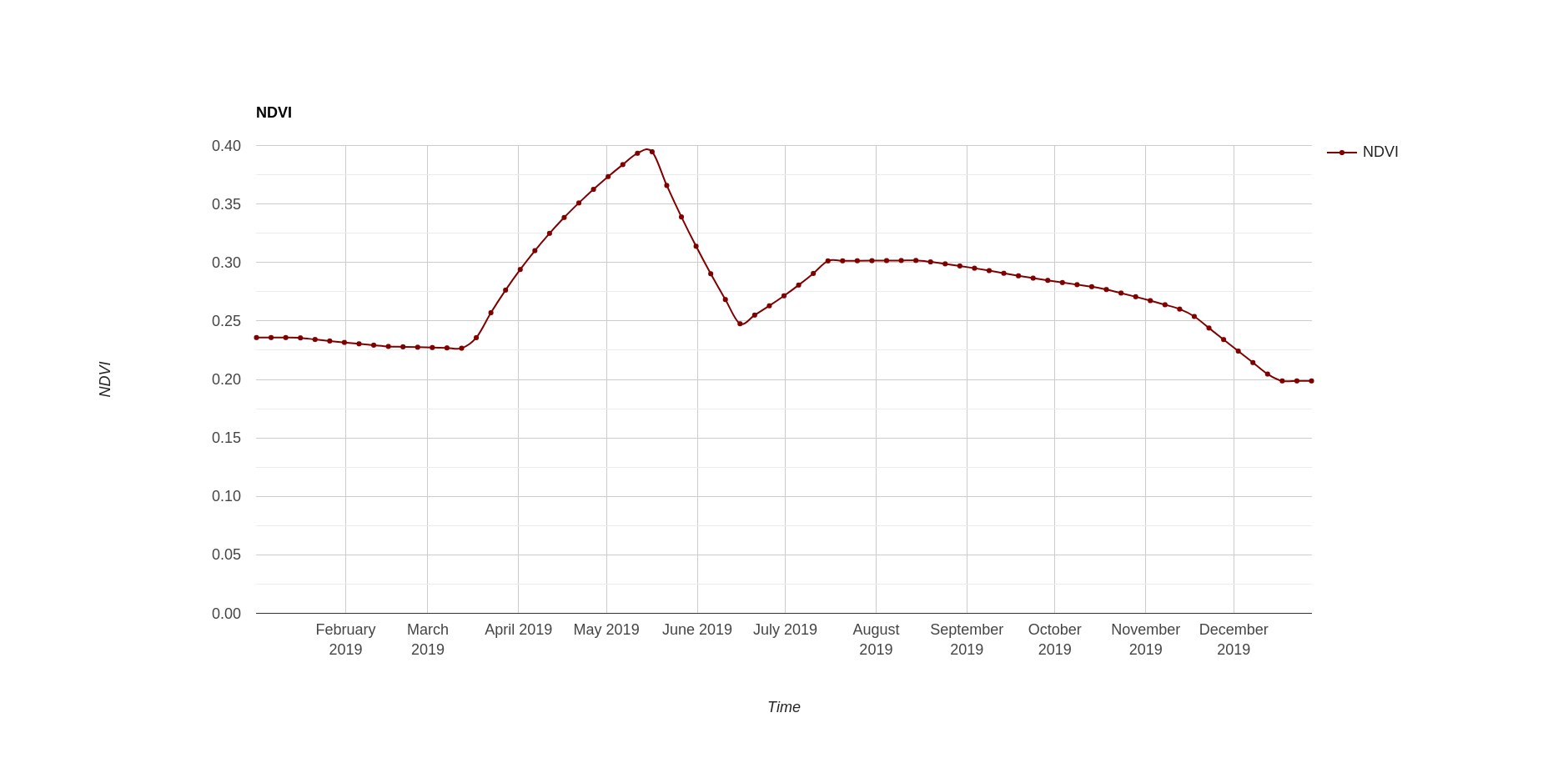
NDVI interpolated time series from monthly to 5 days temporal resolution

4. High resolution biophysical variable retrieval

Estimating biophysical variables is at the core of remote sensing science, allowing close monitoring of crops and forests. Deriving temporally resolved and spatially explicit maps of these variables of interest have been the subject of intense research. This section shows how to generate an animated GIF of one key biophysical variable, the Leaf Area Index (LAI), using HISTARFM data. The LAI measures the total area of leaves per unit ground area and is directly related to the amount of light plants can intercept. To estimate the LAI, we have used the BioNet algorithm from Martinez-Ferrer et al. 2022. BioNet provides new high resolution products of several key variables to quantify the terrestrial biosphere at 30 m Landsat spatial resolution:

Leaf Area Index (LAI)
Fraction of Absorbed Photosynthetically Active Radiation (FAPAR)
Canopy Water Content (CWC)
Fractional Vegetation Cover (FVC)

The following section has three subsections: Biophysical parameter retrieval, map and chart visualization, and GIF generation.

a. Biophysical parameter retrieval

We are going to calculate the LAI from GF_Landsat obtained in section 3.b. Other parameters like the fraction of absorbed photosynthetically active radiation (fAPAR) are also possible to calculate, just changing the variable par from 'LAI' to 'FAPAR'. This code requires using the bioNet repository to compute the biophysical parameter, which is available for all GEE users. You can add the repository to your Code Editor by clicking here.

// Include the bioNet repository.
var bioNet = require('users/ispguv/BioNet:Code/bioNet_nested.js').bioNet;

// Apply the created method to compute the LAI parameter.
var par = 'LAI';
var lai = bioNet.bioNetcompute(GF_Landsat, par);

If you use bioNet, please considering to cite it as follow:

Martínez-Ferrer, L. Moreno-Martínez, Á., Campos-Taberner, M., García-Haro, F. J., Muñoz-Marí, J., Running, S. W., Kimball J., Clinton, N. & Camps-Valls, G. (2022). Quantifying uncertainty in high resolution biophysical variable retrieval with machine learning. Remote Sensing of Environment, 280, 113199.

b. Visualization

To visualize the LAI map, the palette and the visualization parameters are defined for the LAI and its uncertainty. Additionally to the visualization map, a chart of the LAI temporal series in the geometry defined in section 3.c is added to the bottom left part in the map.

// Define color palette and value ranges.
var colors = [
  'ffffe5', 'f7fcb9', 'd9f0a3', 'addd8e', '78c679', '41ab5d', '238443',
  '006837', '004529'
];
var vis_vi_dp = {min: 0, max: 5, palette: colors};
var vis_vi_dp_err = {
  min: 0.0,
  max: 1,
  palette: ['fef0d9', 'fdcc8a', 'fc8d59', 'e34a33', 'b30000']
};

// LAI and its uncertanty maps.
Map.addLayer(lai.select(par), vis_vi_dp, par, true);
Map.addLayer(
    lai.select(par.concat('total')), vis_vi_dp_err, par.concat('_err'), true);

// Select a location in a cropland area in Spain.
var point = ee.Geometry.Point([-0.4600542766311655, 39.24615305773666]);

// Plot the temporal profile; create an image time series chart.
var chart = ui.Chart.image
                .series({
                  imageCollection: lai.select(par),
                  region: point,
                  reducer: ee.Reducer.first(),
                  scale: 30
                })
                .setOptions({
                  title: 'LAI temporal profile',
                  vAxis: {title: 'LAI'},
                  hAxis: {title: 'Time'},
                  series: {
                    0: {
                      color: '008000',
                      lineWidth: 2,
                      pointSize: 4,
                      curveType: 'function'
                    }
                  }
                });

// Add the chart to the map.
chart.style().set({position: 'bottom-left', width: '300px', height: '200px'});
Map.add(chart);

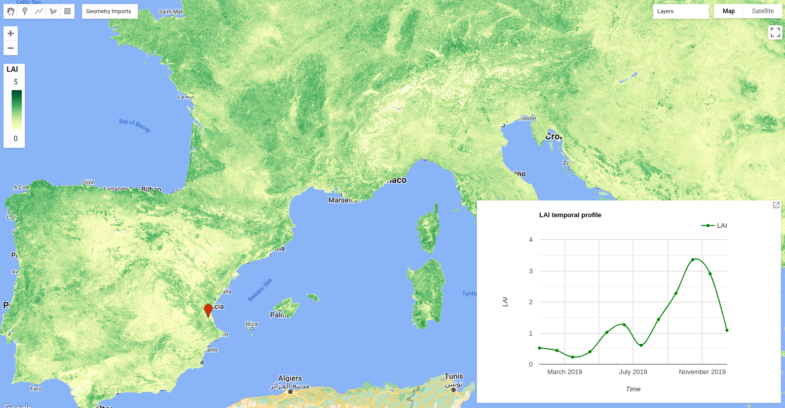
Computed LAI over Europe and temporal profile for a region in Spain

c. Yearly LAI animation (GIF format)

The text added over the GIF is done using the Gennadii Donchyts packages text and style from the available repository for all GEE users. With this repository, the DOY and the year is added to the images. They require a position in the image, a scale and size and color of the text. Additionally, the visualization parameters of the LAI are defined. All variables are used in the function called gifImages to obtain the ImageCollection to visualize in the GIF. After that, the GIF parameters are defined to obtain the GIF visualization using the function ui.Thumbnail, which is added in the map.

// Include text and style repositories.
var text = require('users/gena/packages:text');
var style = require('users/gena/packages:style');

// Get text location for the DOY and the year.
var reg = ee.Geometry.Polygon(
    [[
      [-10.787367805584234, 71.26575224248047],
      [-10.787367805584234, 34.76021219655947],
      [41.41966344441577, 34.76021219655947],
      [41.41966344441577, 71.26575224248047]
    ]],
    null, false);
var pt_doy = text.getLocation(reg, 'right', '5%', '96%');
var pt_year = text.getLocation(reg, 'right', '2%', '65%');
var scale = 4500;
var textProperties = {fontSize: 64, textColor: 'ffffff'};
var visParams =
    {'opacity': 1, 'bands': [par], 'min': 0, 'max': 6, 'palette': colors};

// Create RGB visualization images for use as animation frames.
function gifImages(img) {
  var label = text.draw(
      ee.Date(img.get('system:time_start')).get('year'), pt_year, scale,
      textProperties);
  var label2 = text.draw(img.get('day'), pt_doy, scale, textProperties);
  return img.visualize(visParams).blend(label).blend(label2);
}
var LAIvis = lai.select(par).map(gifImages);

// Generate animation.
var gifParams = {
  'region': reg,
  'dimensions': 512,
  'crs': 'EPSG:4326',
  'framesPerSecond': 2,
  'format': 'gif'
};
Map.add(ui.Thumbnail(
    ee.ImageCollection(LAIvis), gifParams, null, {position: 'bottom-right'}));

Once the animation appears in the map, you can download the image by right-clicking on it.

Resulting LAI animation from interpolated and gap-free HISTARFM data

Now you know how to work with HISTARFM database and few tips of what you can do with it. Hope you like the gap-filled database and you use it in your research and work. If so, please, cite us as follow:

Moreno-Martínez, Á., Izquierdo-Verdiguier, E., Maneta, M. P., Camps-Valls, G., Robinson, N., Muñoz-Marí, J., Sedano, F., Clinton, N. & Running, S. W. (2020). Multispectral high resolution sensor fusion for smoothing and gap-filling in the cloud. Remote Sensing of Environment, 247, 111901.

Acknowledgements

Emma Izquierdo-Verdiguier and Alvaro Moreno-Martinez devised and directed tutorial development. Jordi Muñoz-Marí assisted in the method implementation. All authors contributed text, code and analysis examples.

The tutorial authors would like to thank all the bioNet and HISTARFM creators and Gennadii Donchyts from Deltares for his routines, text, and style, which have been used in this tutorial. Also, we would like to thank the broad Google Earth Engine community for their help and comments. Special thanks to Nicolas Clinton from Google Inc. for actively supporting us during these years.