Page Summary
-
Data converters are client-side capabilities in Earth Engine that allow converting data from methods like
getPixels,computePixels,listFeatures, andcomputeFeaturesinto Python-native formats such as NumPy arrays, Pandas DataFrames, or GeoPandas GeoDataFrames. -
Data converters use the interactive processing environment, which is optimized for small, quick requests and has limits on size and compute time, so consider using the batch processing environment for larger data exports.
-
Common uses for data converters include fetching many small image tiles in parallel for tasks like ML model training and automated workflows, as well as for visualization and data exploration with Python libraries.
-
Earth Engine data can be either "computed" data, generated on the fly, or "stored" data, which exists as assets in catalogs or projects.
-
Data converters offer functions specific to computed and stored data types, such as
ee.data.computeFeaturesandee.data.computePixelsfor computed data, andee.data.listFeaturesandee.data.getPixelsfor stored data.
 View source on GitHub
Data converters are client-side conversion capabilities built into getPixels, computePixels, listFeatures, and computeFeatures. By specifying a compatible fileFormat, these methods can return data in Python-native formats like structured NumPy arrays for rasters and Pandas DataFrames or GeoPandas GeoDataFrames for vectors. In the case of vectors, the listFeatures and computeFeatures methods will make several network requests to fetch all the pages of the table before returning the Python object.
All of these methods transfer data from Earth Engine servers to a client machine using the interactive processing environment, which is optimized for answering small requests quickly. As such, it enforces limits on request size and compute time. You'll need to keep this in mind as you're coding your analysis and decide whether exporting data using the batch processing environment would be better. For example, see ee.data.computePixel limits in the reference docs.
Some common use cases for data converters are fetching many small image tiles in parallel (e.g., training ML models or automated serial workflows) and for visualization and data exploration with your favorite Python libraries. This notebook focuses on data exploration and visualization; if you're interested in learning about fetching data in parallel, see the Medium blog post "Pixels to the people!".
Setup
Import libraries and authenticate to Earth Engine and initialize the API.
import altair as alt
import ee
import eerepr
import geopandas as gpd
import matplotlib.pyplot as plt
import numpy as np
import pandas as pd
from mpl_toolkits.axes_grid1 import ImageGrid
ee.Authenticate()
ee.Initialize(project='my-project')
Data
In this notebook we'll be looking at watersheds in Washington state (USA) and long-term climate averages.
Define asset paths for basins, state boundaries, and climate averages.
BASINS_ID = 'WWF/HydroSHEDS/v1/Basins/hybas_6'
BOUNDARIES_ID = 'FAO/GAUL/2015/level1'
CLIMATE_ID = 'WORLDCLIM/V1/MONTHLY'
Import the basins asset and subset watersheds that intersect Washington state. The result is a ee.FeatureCollection.
basins = ee.FeatureCollection(BASINS_ID)
wa = ee.FeatureCollection(BOUNDARIES_ID).filter(
    'ADM0_NAME == "United States of America" && '
    'ADM1_NAME == "Washington"'
)

wa_basins = basins.filterBounds(wa)
Import the WorldClim climate image collection (each image is the average historical climate for a month), subset the precipitation band and stack the individual images into a single image (each band represents a historical monthly mean). Inspect the resulting ee.Image band names to see that bands are named like prec_month_01 and prec_month_02, indicating mean precipitation for January and February, respectively.
precip = ee.ImageCollection(CLIMATE_ID).select('prec')

months = precip.aggregate_array('month').getInfo()

band_names = [f'prec_month_{str(m).zfill(2)}' for m in months]

monthly_precip = ee.Image(precip.toBands().rename(band_names))

monthly_precip.bandNames()
<ee.ee_list.List at 0x7f1d49d37d40>
Calculate historical mean monthly precipitation for each Washington watershed. These zonal statistics are added as attributes to the wa_basins feature collection.
wa_basins = monthly_precip.reduceRegions(
    collection=wa_basins,
    reducer=ee.Reducer.mean(),
    scale=1e3
)
Converters
In the following sections we'll convert the Earth Engine objects defined above into Python-native formats for visualization and exploring. A distinction is made between computed and stored Earth Engine data because data converter functions are specific to each type.
Computed Earth Engine data
Computed Earth Engine data are those that are generated on the fly through instantiation of non-asset data, computation, or manipulation; they are not stored on disk for later retrieval. To request conversion of computed data, you can use the ee.data.computeFeatures and ee.data.computePixels functions for ee.FeatureCollection and ee.Image objects, respectively.
FeatureCollection to Pandas DataFrame
An ee.FeatureCollection is Earth Engine's table data type. Each ee.Feature in the collection can be thought of as a row and each of its properties as a column - one column stores the geometry. The EE API has a rich set of methods for working with feature collections, but feature collections are difficult to view as a table and you may prefer to use Pandas for analysis. We can transfer the data client-side as a Pandas DataFrame.
We can print the head of the Washington watersheds feature collection to preview the table, but the JSON structure makes it hard to interpret and conceptualize as a table (even with the help of eerep for rich object representation).
wa_basins.limit(5)
<ee.featurecollection.FeatureCollection at 0x7f1d49271bb0>
Use the ee.data.computeFeatures with the fileFormat parameter set to 'PANDAS_DATAFRAME' to get the data as a Pandas DataFrame.
wa_basins_df = ee.data.computeFeatures({
    'expression': wa_basins,
    'fileFormat': 'PANDAS_DATAFRAME'
})
Print the object's type and see that it is pandas.core.frame.DataFrame. Printing the head of the object shows the nicely formatted table.
display(type(wa_basins_df))
wa_basins_df.head()
pandas.DataFrame
Now we can use Pandas syntax to convert the wide table into a long table so that month is a factor and precipitation is a variable.
wa_basins_df = wa_basins_df.melt(
    id_vars=["HYBAS_ID"],
    value_vars=band_names,
    var_name="Month",
    value_name="Precipitation",
)
wa_basins_df
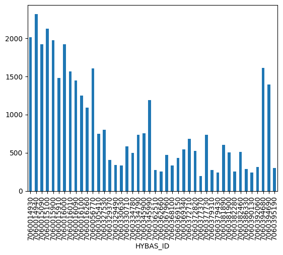
We can use Pandas' groupby method and built-in matplotlib charting wrappers for a quick look at mean total annual precipition for each watershed.
wa_basins_df.groupby(['HYBAS_ID'])['Precipitation'].sum().plot.bar()
<Axes: xlabel='HYBAS_ID'>
There are lots of charting libraries for visualizing DataFrame objects. Here, we plot the data with Altair using a stacked column chart to show the total mean annual precipitation (by monthly contribution) for each watershed intersecting Washington state. We can see quite a range in total precipitation and that summer months are generally drier than other months.
alt.Chart(wa_basins_df).mark_bar().encode(
    x=alt.X('HYBAS_ID:O'),
    y=alt.Y('Precipitation:Q', title='Precipitation (mm)'),
    color=alt.Color('Month', scale=alt.Scale(scheme='rainbow')),
    tooltip=alt.Tooltip(['HYBAS_ID', 'Precipitation', 'Month'])
).interactive()
FeatureCollection to GeoPandas GeoDataFrame
Use the ee.data.computeFeatures with the fileFormat parameter set to 'GEOPANDAS_GEODATAFRAME' to get the Washington basins climate data as a GeoPandas GeoDataFrame. It allows you to use the table manipulation and querying functions of Pandas, in addition to geospatial operations and visualizations.
wa_basins_gdf = ee.data.computeFeatures({
    'expression': wa_basins,
    'fileFormat': 'GEOPANDAS_GEODATAFRAME'
})

# Need to set the CRS.
# Make sure it matches the CRS of FeatureCollection geometries.
wa_basins_gdf.crs = 'EPSG:4326'

display(type(wa_basins_gdf))
wa_basins_gdf.head()
geopandas.geodataframe.GeoDataFrame
Fetch the Washington state boundary as GeoDataFrame too.
wa_gdf = ee.data.computeFeatures({
    'expression': wa,
    'fileFormat': 'GEOPANDAS_GEODATAFRAME'
})

wa_gdf.crs = 'EPSG:4326'
Clip the watershed geometries by the Washington state boundary using the GeoDataFrame.clip method and convert the original mercator projection to a Washington-specific projection for better visualization.
wa_basins_gdf = wa_basins_gdf.clip(wa_gdf).to_crs(2856)
Sum the 12 months of mean precipitation for each watershed and append the values in a new column called prec_total.
wa_basins_gdf['prec_total'] = wa_basins_gdf[band_names].sum(axis=1)
wa_basins_gdf.head()
Use matplotlib to plot a choropleth map of mean annual precipitation by watershed and highlight the watershed with the minimum precipitation using a red border.
# Define the choropleth map.
ax = wa_basins_gdf.plot(
    column='prec_total',
    cmap='viridis_r',
    vmin=wa_basins_gdf['prec_total'].min(),
    vmax=wa_basins_gdf['prec_total'].max(),
    legend=False,
    edgecolor='grey', linewidth=0.5
)

# Highlight the basin with the minimum annual precipitation: subset the geometry
# with the minimum precipitation total and then add it to the basin
# precipitation plot.
min_prec_gdf = wa_basins_gdf.loc[[wa_basins_gdf['prec_total'].idxmin()]]
min_prec_gdf.plot(ax=ax, color='none', edgecolor='red', linewidth=2)

# Add axis labels, a colorbar, and rotate x axis ticks.
ax.set_xlabel('Eastings [m]')
ax.set_ylabel('Northings [m]')
colorbar = plt.colorbar(ax.get_children()[0], fraction=0.03)
colorbar.set_label('Precipitation (mm)')
plt.xticks(rotation=45)

plt.show()
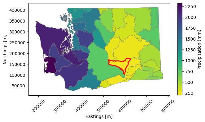
Image to NumPy structured array
Here we use ee.data.computePixels to request the monthly_precip computed Earth Engine image (each band is mean precipitation for a given month) as a NumPy structured array. It is a global dataset, so we'll request only the Washington state basins bounding region at a resolution of 1500 meters. We can use the ee.Image.clipToBoundsAndScale function to do this, which is a convenient alternative to supplying the grid argument.
monthly_precip_washington = monthly_precip.clipToBoundsAndScale(
    geometry=wa_basins, scale=1500
)

monthly_precip_npy = ee.data.computePixels({
    'expression': monthly_precip_washington,
    'fileFormat': 'NUMPY_NDARRAY'
})

monthly_precip_npy
array([[( 1.51e+02,  1.07e+02,  9.5e+01,  6.7e+01,  6.1e+01,  5.7e+01,  5.6e+01,  5.1e+01,  6.6e+01,  1.29e+02,  1.51e+02,  1.52e+02),
        ( 1.49e+02,  1.05e+02,  9.2e+01,  6.5e+01,  6.0e+01,  5.5e+01,  5.4e+01,  4.9e+01,  6.6e+01,  1.33e+02,  1.52e+02,  1.50e+02),
        ( 1.49e+02,  1.06e+02,  9.5e+01,  6.7e+01,  6.1e+01,  5.7e+01,  5.6e+01,  5.1e+01,  6.6e+01,  1.26e+02,  1.49e+02,  1.51e+02),
        ...,
        ( 2.60e+01,  2.40e+01,  2.5e+01,  4.0e+01,  5.8e+01,  8.5e+01,  5.9e+01,  5.5e+01,  4.6e+01,  2.30e+01,  2.00e+01,  2.50e+01),
        ( 2.50e+01,  2.40e+01,  2.4e+01,  3.9e+01,  5.7e+01,  8.5e+01,  5.9e+01,  5.5e+01,  4.6e+01,  2.20e+01,  1.90e+01,  2.40e+01),
        ( 2.50e+01,  2.40e+01,  2.4e+01,  3.9e+01,  5.7e+01,  8.5e+01,  5.9e+01,  5.5e+01,  4.6e+01,  2.20e+01,  1.90e+01,  2.40e+01)],
       [( 1.51e+02,  1.06e+02,  9.4e+01,  6.6e+01,  6.0e+01,  5.6e+01,  5.4e+01,  5.0e+01,  6.6e+01,  1.36e+02,  1.55e+02,  1.53e+02),
        ( 1.50e+02,  1.05e+02,  9.2e+01,  6.5e+01,  6.0e+01,  5.5e+01,  5.3e+01,  4.9e+01,  6.6e+01,  1.39e+02,  1.56e+02,  1.52e+02),
        ( 1.54e+02,  1.08e+02,  9.2e+01,  6.6e+01,  6.1e+01,  5.5e+01,  5.2e+01,  4.9e+01,  6.8e+01,  1.54e+02,  1.65e+02,  1.57e+02),
        ...,
        ( 2.70e+01,  2.50e+01,  2.5e+01,  4.0e+01,  5.8e+01,  8.5e+01,  5.9e+01,  5.5e+01,  4.6e+01,  2.30e+01,  2.00e+01,  2.50e+01),
        ( 2.60e+01,  2.40e+01,  2.5e+01,  4.0e+01,  5.8e+01,  8.5e+01,  5.9e+01,  5.5e+01,  4.6e+01,  2.30e+01,  1.90e+01,  2.50e+01),
        ( 2.60e+01,  2.40e+01,  2.5e+01,  4.0e+01,  5.8e+01,  8.5e+01,  5.9e+01,  5.5e+01,  4.6e+01,  2.20e+01,  1.90e+01,  2.50e+01)],
       [( 1.53e+02,  1.08e+02,  9.3e+01,  6.6e+01,  6.1e+01,  5.5e+01,  5.3e+01,  4.9e+01,  6.7e+01,  1.48e+02,  1.61e+02,  1.56e+02),
        ( 1.51e+02,  1.06e+02,  9.3e+01,  6.5e+01,  6.0e+01,  5.5e+01,  5.3e+01,  4.9e+01,  6.6e+01,  1.40e+02,  1.56e+02,  1.53e+02),
        ( 1.58e+02,  1.12e+02,  9.5e+01,  6.8e+01,  6.3e+01,  5.7e+01,  5.2e+01,  5.0e+01,  7.0e+01,  1.62e+02,  1.72e+02,  1.63e+02),
        ...,
        ( 2.70e+01,  2.50e+01,  2.6e+01,  4.1e+01,  5.9e+01,  8.6e+01,  5.9e+01,  5.5e+01,  4.7e+01,  2.30e+01,  2.00e+01,  2.60e+01),
        ( 2.60e+01,  2.40e+01,  2.5e+01,  4.0e+01,  5.8e+01,  8.5e+01,  5.9e+01,  5.5e+01,  4.6e+01,  2.30e+01,  1.90e+01,  2.50e+01),
        ( 2.60e+01,  2.40e+01,  2.5e+01,  4.0e+01,  5.8e+01,  8.5e+01,  5.9e+01,  5.5e+01,  4.6e+01,  2.20e+01,  1.90e+01,  2.50e+01)],
       ...,
       [(-3.40e+38, -3.40e+38, -3.4e+38, -3.4e+38, -3.4e+38, -3.4e+38, -3.4e+38, -3.4e+38, -3.4e+38, -3.40e+38, -3.40e+38, -3.40e+38),
        (-3.40e+38, -3.40e+38, -3.4e+38, -3.4e+38, -3.4e+38, -3.4e+38, -3.4e+38, -3.4e+38, -3.4e+38, -3.40e+38, -3.40e+38, -3.40e+38),
        (-3.40e+38, -3.40e+38, -3.4e+38, -3.4e+38, -3.4e+38, -3.4e+38, -3.4e+38, -3.4e+38, -3.4e+38, -3.40e+38, -3.40e+38, -3.40e+38),
        ...,
        ( 5.80e+01,  4.10e+01,  3.3e+01,  2.6e+01,  3.4e+01,  3.2e+01,  1.4e+01,  1.7e+01,  2.0e+01,  2.00e+01,  4.40e+01,  5.80e+01),
        ( 5.60e+01,  4.00e+01,  3.2e+01,  2.5e+01,  3.3e+01,  3.1e+01,  1.3e+01,  1.7e+01,  1.9e+01,  1.90e+01,  4.30e+01,  5.50e+01),
        ( 5.50e+01,  3.90e+01,  3.2e+01,  2.5e+01,  3.3e+01,  3.0e+01,  1.3e+01,  1.6e+01,  1.9e+01,  1.90e+01,  4.20e+01,  5.50e+01)],
       [(-3.40e+38, -3.40e+38, -3.4e+38, -3.4e+38, -3.4e+38, -3.4e+38, -3.4e+38, -3.4e+38, -3.4e+38, -3.40e+38, -3.40e+38, -3.40e+38),
        (-3.40e+38, -3.40e+38, -3.4e+38, -3.4e+38, -3.4e+38, -3.4e+38, -3.4e+38, -3.4e+38, -3.4e+38, -3.40e+38, -3.40e+38, -3.40e+38),
        (-3.40e+38, -3.40e+38, -3.4e+38, -3.4e+38, -3.4e+38, -3.4e+38, -3.4e+38, -3.4e+38, -3.4e+38, -3.40e+38, -3.40e+38, -3.40e+38),
        ...,
        ( 5.50e+01,  3.90e+01,  3.2e+01,  2.5e+01,  3.2e+01,  3.0e+01,  1.3e+01,  1.6e+01,  1.9e+01,  1.90e+01,  4.30e+01,  5.50e+01),
        ( 5.60e+01,  4.00e+01,  3.2e+01,  2.5e+01,  3.3e+01,  3.1e+01,  1.3e+01,  1.7e+01,  1.9e+01,  1.90e+01,  4.30e+01,  5.60e+01),
        ( 5.50e+01,  3.90e+01,  3.2e+01,  2.5e+01,  3.3e+01,  3.0e+01,  1.3e+01,  1.6e+01,  1.9e+01,  1.90e+01,  4.30e+01,  5.50e+01)],
       [(-3.40e+38, -3.40e+38, -3.4e+38, -3.4e+38, -3.4e+38, -3.4e+38, -3.4e+38, -3.4e+38, -3.4e+38, -3.40e+38, -3.40e+38, -3.40e+38),
        (-3.40e+38, -3.40e+38, -3.4e+38, -3.4e+38, -3.4e+38, -3.4e+38, -3.4e+38, -3.4e+38, -3.4e+38, -3.40e+38, -3.40e+38, -3.40e+38),
        (-3.40e+38, -3.40e+38, -3.4e+38, -3.4e+38, -3.4e+38, -3.4e+38, -3.4e+38, -3.4e+38, -3.4e+38, -3.40e+38, -3.40e+38, -3.40e+38),
        ...,
        ( 5.70e+01,  4.00e+01,  3.3e+01,  2.6e+01,  3.3e+01,  3.1e+01,  1.4e+01,  1.7e+01,  1.9e+01,  2.00e+01,  4.40e+01,  5.70e+01),
        ( 5.30e+01,  3.80e+01,  3.1e+01,  2.4e+01,  3.2e+01,  2.9e+01,  1.2e+01,  1.5e+01,  1.8e+01,  1.80e+01,  4.20e+01,  5.30e+01),
        ( 5.30e+01,  3.80e+01,  3.1e+01,  2.4e+01,  3.1e+01,  2.9e+01,  1.2e+01,  1.5e+01,  1.8e+01,  1.80e+01,  4.20e+01,  5.30e+01)]],
      shape=(556, 834), dtype=[('prec_month_01', '<f4'), ('prec_month_02', '<f4'), ('prec_month_03', '<f4'), ('prec_month_04', '<f4'), ('prec_month_05', '<f4'), ('prec_month_06', '<f4'), ('prec_month_07', '<f4'), ('prec_month_08', '<f4'), ('prec_month_09', '<f4'), ('prec_month_10', '<f4'), ('prec_month_11', '<f4'), ('prec_month_12', '<f4')])
NumPy structured arrays work well for multiband image data. You can think of them as a table of arrays where each band is a column accessible from a field (band) name. It also permits each band to have a different data type.
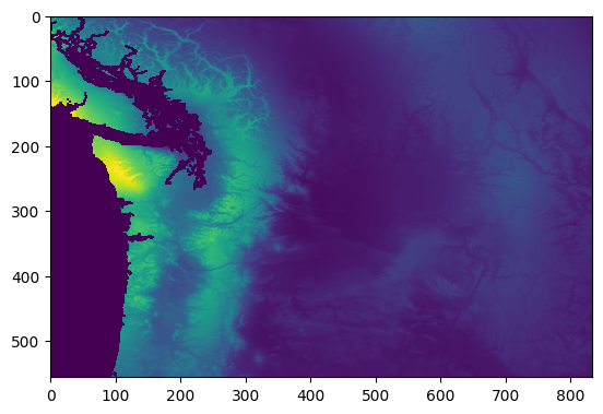
For example, get the list of field (band) names and then subset an array by name and print its shape and display a preview of it.
names = monthly_precip_npy.dtype.names
print('field names:', names)

prec_month_10_arr = monthly_precip_npy['prec_month_10']
print('Selected array (band) shape:', prec_month_10_arr.shape)
display(prec_month_10_arr)
plt.imshow(prec_month_10_arr, vmin=0, vmax=320)
field names: ('prec_month_01', 'prec_month_02', 'prec_month_03', 'prec_month_04', 'prec_month_05', 'prec_month_06', 'prec_month_07', 'prec_month_08', 'prec_month_09', 'prec_month_10', 'prec_month_11', 'prec_month_12')
Selected array (band) shape: (556, 834)
array([[ 1.29e+02,  1.33e+02,  1.26e+02, ...,  2.30e+01,  2.20e+01,
         2.20e+01],
       [ 1.36e+02,  1.39e+02,  1.54e+02, ...,  2.30e+01,  2.30e+01,
         2.20e+01],
       [ 1.48e+02,  1.40e+02,  1.62e+02, ...,  2.30e+01,  2.30e+01,
         2.20e+01],
       ...,
       [-3.40e+38, -3.40e+38, -3.40e+38, ...,  2.00e+01,  1.90e+01,
         1.90e+01],
       [-3.40e+38, -3.40e+38, -3.40e+38, ...,  1.90e+01,  1.90e+01,
         1.90e+01],
       [-3.40e+38, -3.40e+38, -3.40e+38, ...,  2.00e+01,  1.80e+01,
         1.80e+01]], shape=(556, 834), dtype=float32)
<matplotlib.image.AxesImage at 0x7f1d48d9e390>
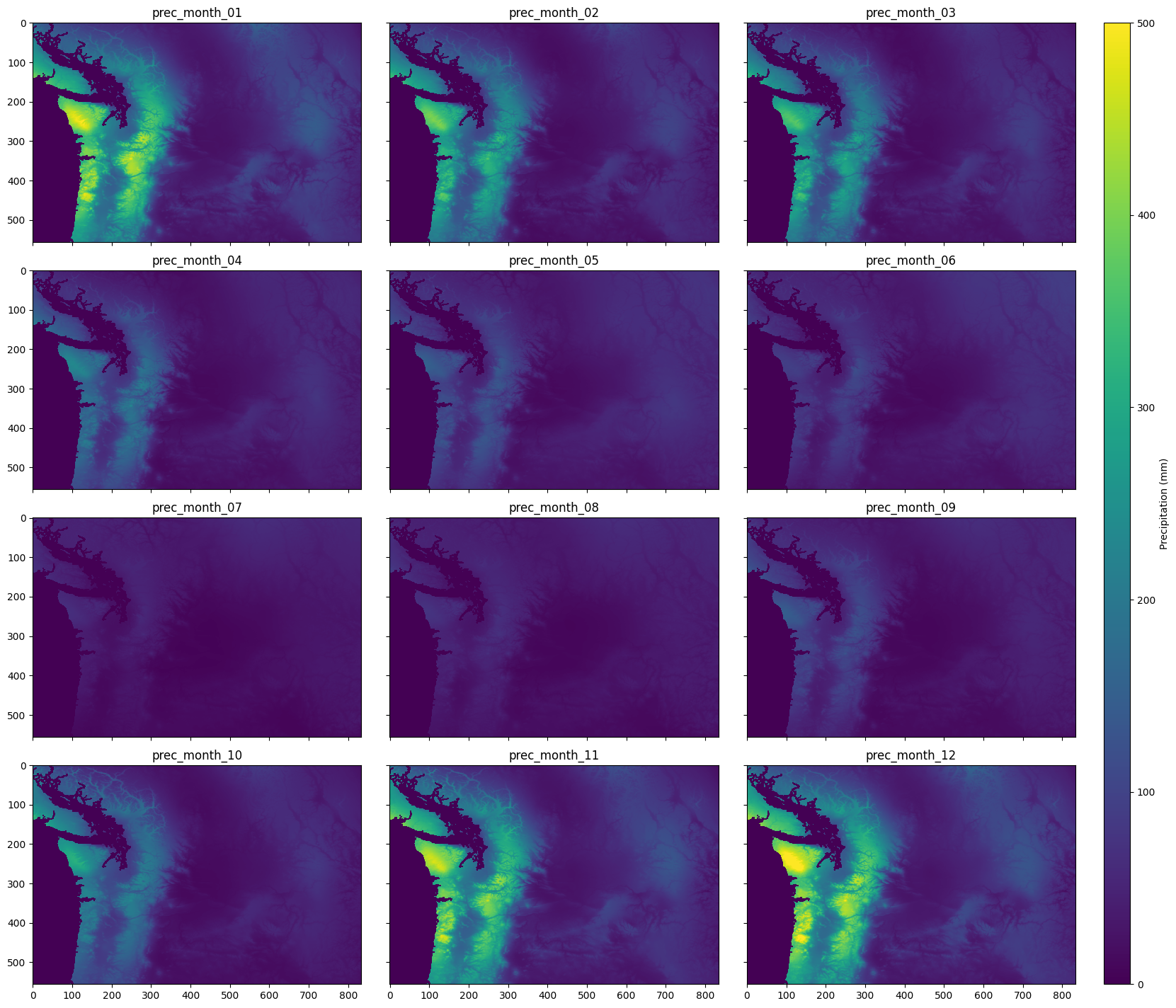
Since we have all months of mean precipitation, we can use the matplotlib ImageGrid function to show a time series grid for simple visual interpolation of intra-annual precipitation patterns.
# Set up the figure and grid.
fig = plt.figure(figsize=(20.0, 20.0))
grid = ImageGrid(
    fig,
    111,
    nrows_ncols=(4, 3),
    axes_pad=0.4,
    cbar_mode="single",
    cbar_location="right",
    cbar_pad=0.4,
    cbar_size="2%",
)

# Display each band to a grid cell.
for ax, name in zip(grid, names):
    ax.imshow(monthly_precip_npy[name], vmin=0, vmax=500)
    ax.set_title(name)

# Add colorbar.
colorbar = plt.colorbar(ax.get_children()[0], cax=grid[0].cax)
colorbar.set_label("Precipitation (mm)")

plt.show()
Stored Earth Engine data
Stored Earth Engine data are those that exist as assets in the public data catalog or personal and shared cloud projects. To request conversion of stored data, you can use the ee.data.listFeatures and ee.data.getPixels functions for ee.FeatureCollection and ee.Image objects, respectively.
FeatureCollection to Pandas DataFrame
We use the ee.data.listFeatures function to get a Pandas DataFrame from a stored FeatureCollection asset. The process is similar to converting a computed FeatureCollection (see above), but since we can't manipulate the FeatureCollection there are extra parameters to optionally specify the region and filter by property values. In this case, we subset the global watershed dataset to those that intersect Washington state using the region parameter and apply a filter to only include watersheds that are greater than or equal to river order 3, using the filter parameter.
high_order_wa_basins_df = ee.data.listFeatures({
    'assetId': 'WWF/HydroSHEDS/v1/Basins/hybas_6',
    'region': wa.geometry().getInfo(),
    'filter': 'ORDER >= 3',
    'fileFormat': 'PANDAS_DATAFRAME'
})

high_order_wa_basins_df
FeatureCollection to GeoPandas GeoDataFrame
If we change the fileFormat argument to 'GEOPANDAS_GEODATAFRAME', we'll get a GeoPandas GeoDataFrame.
high_order_wa_basins_gdf = ee.data.listFeatures({
    'assetId': 'WWF/HydroSHEDS/v1/Basins/hybas_6',
    'region': wa.geometry().getInfo(),
    'filter': 'ORDER >= 3',
    'fileFormat': 'GEOPANDAS_GEODATAFRAME'
})

display(type(wa_basins_gdf))
high_order_wa_basins_gdf
geopandas.geodataframe.GeoDataFrame
Display the high order watersheds in Washington with its border so we can see their location in the state.
# Create an initial plot with the high river order watersheds.
ax = high_order_wa_basins_gdf.plot(edgecolor='purple', linewidth=1)

# Overlay the Washington state border for context.
wa_gdf.plot(ax=ax, color='none', edgecolor='black', linewidth=1)

# Set axis labels.
ax.set_xlabel('Eastings [degrees]')
ax.set_ylabel('Northings [degrees]')

plt.show()
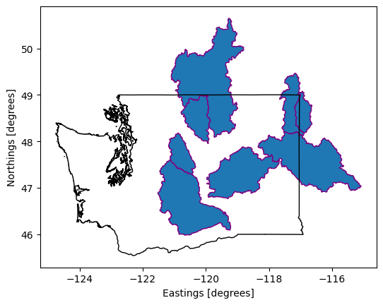
Image to NumPy structured array
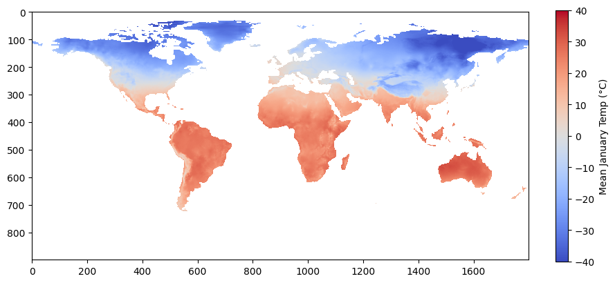
Here we use ee.data.getPixels to request the global historical average temperature for January (according to the WorldClim data) as a NumPy structured array. Unlike ee.data.computePixels (above), we can't use the very convenient ee.Image.clipToBoundsAndScale function to define the request region and scale because we need to access the asset directly without manipulation. Instead, we have to use the more verbose and less intuitive grid parameter.
The grid argument in our request starts by defining a global 1-degree grid and then applies a scale factor of 5 to get higher resolution.
SCALE_FACTOR = 5

jan_mean_temp_npy = ee.data.getPixels({
    'assetId': 'WORLDCLIM/V1/MONTHLY/01',
    'fileFormat': 'NUMPY_NDARRAY',
    'grid': {
        'dimensions': {
            'width': 360 * SCALE_FACTOR,
            'height': 180 * SCALE_FACTOR
        },
        'affineTransform': {
            'scaleX': 1 / SCALE_FACTOR,
            'shearX': 0,
            'translateX': -180,
            'shearY': 0,
            'scaleY': -1 / SCALE_FACTOR,
            'translateY': 90
        },
        'crsCode': 'EPSG:4326',
    },
    'bandIds': ['tavg']
})

jan_mean_temp_npy
array([[(-3.4e+38,), (-3.4e+38,), (-3.4e+38,), ..., (-3.4e+38,),
        (-3.4e+38,), (-3.4e+38,)],
       [(-3.4e+38,), (-3.4e+38,), (-3.4e+38,), ..., (-3.4e+38,),
        (-3.4e+38,), (-3.4e+38,)],
       [(-3.4e+38,), (-3.4e+38,), (-3.4e+38,), ..., (-3.4e+38,),
        (-3.4e+38,), (-3.4e+38,)],
       ...,
       [(-3.4e+38,), (-3.4e+38,), (-3.4e+38,), ..., (-3.4e+38,),
        (-3.4e+38,), (-3.4e+38,)],
       [(-3.4e+38,), (-3.4e+38,), (-3.4e+38,), ..., (-3.4e+38,),
        (-3.4e+38,), (-3.4e+38,)],
       [(-3.4e+38,), (-3.4e+38,), (-3.4e+38,), ..., (-3.4e+38,),
        (-3.4e+38,), (-3.4e+38,)]],
      shape=(900, 1800), dtype=[('tavg', '<f4')])
Extract the 'tavg' band from the structured array, set the background values as nan, and scale the temperature values to the appropriate range.
jan_mean_temp_npy = jan_mean_temp_npy['tavg']

jan_mean_temp_npy = np.where(jan_mean_temp_npy < -9999, np.nan, jan_mean_temp_npy)
jan_mean_temp_npy = jan_mean_temp_npy * 0.1
jan_mean_temp_npy
array([[nan, nan, nan, ..., nan, nan, nan],
       [nan, nan, nan, ..., nan, nan, nan],
       [nan, nan, nan, ..., nan, nan, nan],
       ...,
       [nan, nan, nan, ..., nan, nan, nan],
       [nan, nan, nan, ..., nan, nan, nan],
       [nan, nan, nan, ..., nan, nan, nan]],
      shape=(900, 1800), dtype=float32)
Plot the 2D array as an image using matplotlib.
fig = plt.figure(figsize=(10., 10.))
ax = plt.imshow(jan_mean_temp_npy, cmap='coolwarm', vmin=-40, vmax=40)

colorbar = plt.colorbar(ax, fraction=0.0235)
colorbar.set_label('Mean January Temp (°C)')

plt.show()