Page Summary
-
Histogram matching is a method to "calibrate" one image to another by transforming its cumulative distribution function (CDF) to match the target image's CDF.
-
The process involves interpolating source image values based on a piecewise-linear function derived from the cumulative histograms of both images.
-
Custom functions are used to generate the lookup table and apply the histogram matching, requiring source and target images and a geometry for histogram calculation.
-
Finding a suitable target image often involves filtering an image collection by date proximity and spatial intersection to the source image.
-
While generally effective, anomalies like clouds can skew the results, and minor mis-registration between images is usually acceptable.
 View source on GitHub
Modified from the Medium blog post by Noel Gorelick
Histogram matching is a quick and easy way to "calibrate" one image to match another. In mathematical terms, it's the process of transforming one image so that the cumulative distribution function (CDF) of values in each band matches the CDF of bands in another image.
To illustrate what this looks like and how it works, I'm going to histogram-match a high-resolution (0.8m/pixel) SkySat image to the Landsat 8 calibrated surface reflectance images taken around the same time. Below is what it looks like with the SkySat image overlaid on top of the Landsat data, before the matching. Each image's histogram is shown as well:
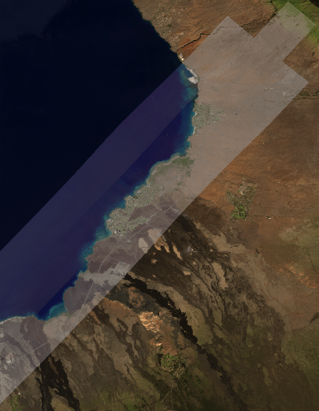
SkySat image swath overlaid on Landsat 8 image
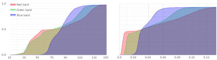
Cumulative histogram for SkySat (left) and Landsat 8 surface reflectance (right).
To make the histograms match, we can interpolate the values from the source image (SkySat) into the range of the target image (Landsat), using a piecewise-linear function that puts the correct ratio of pixels into each bin.
Let's get started: setup the Earth Engine API.
Setup Earth Engine
import ee
import geemap

ee.Authenticate()
ee.Initialize(project='my-project')
Functions
The following is code to generate the piecewise-linear function using the cumulative count histograms of each image.
def lookup(source_hist, target_hist):
    """Creates a lookup table to make a source histogram match a target histogram.

    Args:
        source_hist: The histogram to modify. Expects the Nx2 array format produced by ee.Reducer.autoHistogram.
        target_hist: The histogram to match to. Expects the Nx2 array format produced by ee.Reducer.autoHistogram.

    Returns:
        A dictionary with 'x' and 'y' properties that respectively represent the x and y
        array inputs to the ee.Image.interpolate function.
    """

    # Split the histograms by column and normalize the counts.
    source_values = source_hist.slice(1, 0, 1).project([0])
    source_counts = source_hist.slice(1, 1, 2).project([0])
    source_counts = source_counts.divide(source_counts.get([-1]))

    target_values = target_hist.slice(1, 0, 1).project([0])
    target_counts = target_hist.slice(1, 1, 2).project([0])
    target_counts = target_counts.divide(target_counts.get([-1]))

    # Find first position in target where targetCount >= srcCount[i], for each i.
    def make_lookup(n):
        return target_values.get(target_counts.gte(n).argmax())

    lookup = source_counts.toList().map(make_lookup)

    return {'x': source_values.toList(), 'y': lookup}
This code starts by splitting the (2D Array) histograms into the pixel values (column 0) and pixel counts (column 1), and normalizes the counts by dividing by the total count (the last value).
Next, for each source bin, it finds the index of the first bin in the target histogram where target_count ≥ src_count[i]. To determine that, we compare each value from source_count to the entire array of target_counts. This comparison generates an array of 0s where the comparison is false and 1s where the comparison is true. The index of the first non-zero value can be found using the Array.argmax() function, and using that index, we can determine the target_value that each src_value should be adjusted to. The output of this function is formatted as a dictionary that's suitable for passing directly into the Image.interpolate() function.
Next, here's the code for generating the histograms and adjusting the images.
def histogram_match(source_img, target_img, geometry):
    """Performs histogram matching for 3-band RGB images by forcing the histogram CDF of source_img to match target_img.

    Args:
        source_img: A 3-band ee.Image to be color matched. Must have bands named 'R', 'G', and 'B'.
        target_img: A 3-band ee.Image for color reference. Must have bands named 'R', 'G', and 'B'.
        geometry: An ee.Geometry that defines the region to generate RGB histograms for.
          It should intersect both source_img and target_img inputs.

    Returns:
        A copy of src_img color-matched to target_img.
    """

    args = {
        'reducer': ee.Reducer.autoHistogram(maxBuckets=256, cumulative=True),
        'geometry': geometry,
        'scale': 1, # Need to specify a scale, but it doesn't matter what it is because bestEffort is true.
        'maxPixels': 65536 * 4 - 1,
        'bestEffort': True
    }

    # Only use pixels in target that have a value in source (inside the footprint and unmasked).
    source = source_img.reduceRegion(**args)
    target = target_img.updateMask(source_img.mask()).reduceRegion(**args)

    return ee.Image(ee.Image.cat(
        source_img.select(['R']).interpolate(**lookup(source.getArray('R'), target.getArray('R'))),
        source_img.select(['G']).interpolate(**lookup(source.getArray('G'), target.getArray('G'))),
        source_img.select(['B']).interpolate(**lookup(source.getArray('B'), target.getArray('B')))
    ).copyProperties(source_img, ['system:time_start']))
This code runs a reduceRegion() on each image to generate a cumulative histogram, making sure that only pixels that are in both images are included when computing the histograms (just in case there might be a cloud or something else just outside of the high-res image, that might distort the results). It's not important to generate that histogram with a really high fidelity, so the maxPixels argument is set to use less than "4 tiles" of data (256 * 256 * 4) and bestEffort is turned on, to make the computation run fast. When these arguments are set this way, the reduceRegion() function will try to figure out how many pixels it would need to process at the given scale, and if that's greater than the maxPixels value, it computes a lower scale to keep the total number of pixels below maxPixels. That all means you need to specify a scale, but it doesn't matter what it is as it'll be mostly ignored.
This code then generates the lookup tables for each band in the input image, calls the interpolate() function for each, and combines the results into a single image.
Before the histogram_match function can be used, we need to identify the source and target images. The following function is for finding a target RGB-reference image within a given image collection that is nearest in observation date to the image we want color matched.
def find_closest(target_image, image_col, days):
    """Filter images in a collection by date proximity and spatial intersection to a target image.

    Args:
        target_image: An ee.Image whose observation date is used to find near-date images in
          the provided image_col image collection. It must have a 'system:time_start' property.
        image_col: An ee.ImageCollection to filter by date proximity and spatial intersection
          to the target_image. Each image in the collection must have a 'system:time_start'
          property.
        days: A number that defines the maximum number of days difference allowed between
          the target_image and images in the image_col.

    Returns:
        An ee.ImageCollection that has been filtered to include those images that are within the
          given date proximity to target_image and intersect it spatially.
    """

    # Compute the timespan for N days (in milliseconds).
    range = ee.Number(days).multiply(1000 * 60 * 60 * 24)

    filter = ee.Filter.And(
        ee.Filter.maxDifference(range, 'system:time_start', None, 'system:time_start'),
        ee.Filter.intersects('.geo', None, '.geo'))

    closest = (ee.Join.saveAll('matches', 'measure')
        .apply(ee.ImageCollection([target_image]), image_col, filter))

    return ee.ImageCollection(ee.List(closest.first().get('matches')))
The previous functions are generically useful for performing image histogram matching; they are not specific to any particular image or image collection. They are the building blocks for the procedure.
Application
The following steps are specific to the SkySat-to-Landsat scenario introduced earlier.
First define a region of interest and the source SkySat image to histogram-match to Landsat 8 images; we'll also clip the image by the region of interest.
geometry = ee.Geometry.BBox(-155.971, 19.782, -155.733, 20.09)

skysat = (ee.Image('SKYSAT/GEN-A/PUBLIC/ORTHO/RGB/s01_20161020T214047Z')
    .clip(geometry))
Next prepare a Landsat 8 collection by applying a cloud/shadow mask, scaling, and selecting/renaming RGB bands.
def prep_landsat(image):
    """Scale, apply cloud/shadow mask, and select/rename Landsat 8 bands."""
    qa_mask = image.select('QA_PIXEL').bitwiseAnd(int('11111', 2)).eq(0)

    def get_factor_img(factor_names):
        factor_list = image.toDictionary().select(factor_names).values()
        return ee.Image.constant(factor_list)

    scale_img = get_factor_img(['REFLECTANCE_MULT_BAND_.'])
    offset_img = get_factor_img(['REFLECTANCE_ADD_BAND_.'])
    scaled = image.select('SR_B.').multiply(scale_img).add(offset_img)

    return image.addBands(scaled, None, True).select(
        ['SR_B4', 'SR_B3', 'SR_B2'], ['R', 'G', 'B']).updateMask(qa_mask)

# Get the landsat collection, cloud masked and scaled to surface reflectance.
landsat_col = ee.ImageCollection('LANDSAT/LC08/C02/T1_L2').filterBounds(
    geometry).map(prep_landsat)
Now find the Landsat images within 32 days of the SkySat image, sort the images by cloud cover and then mosaic them. Use the result as the reference image to histogram-match the SkySat image to.
reference = find_closest(skysat, landsat_col, 32).sort('CLOUD_COVER').mosaic()
result = histogram_match(skysat, reference, geometry)
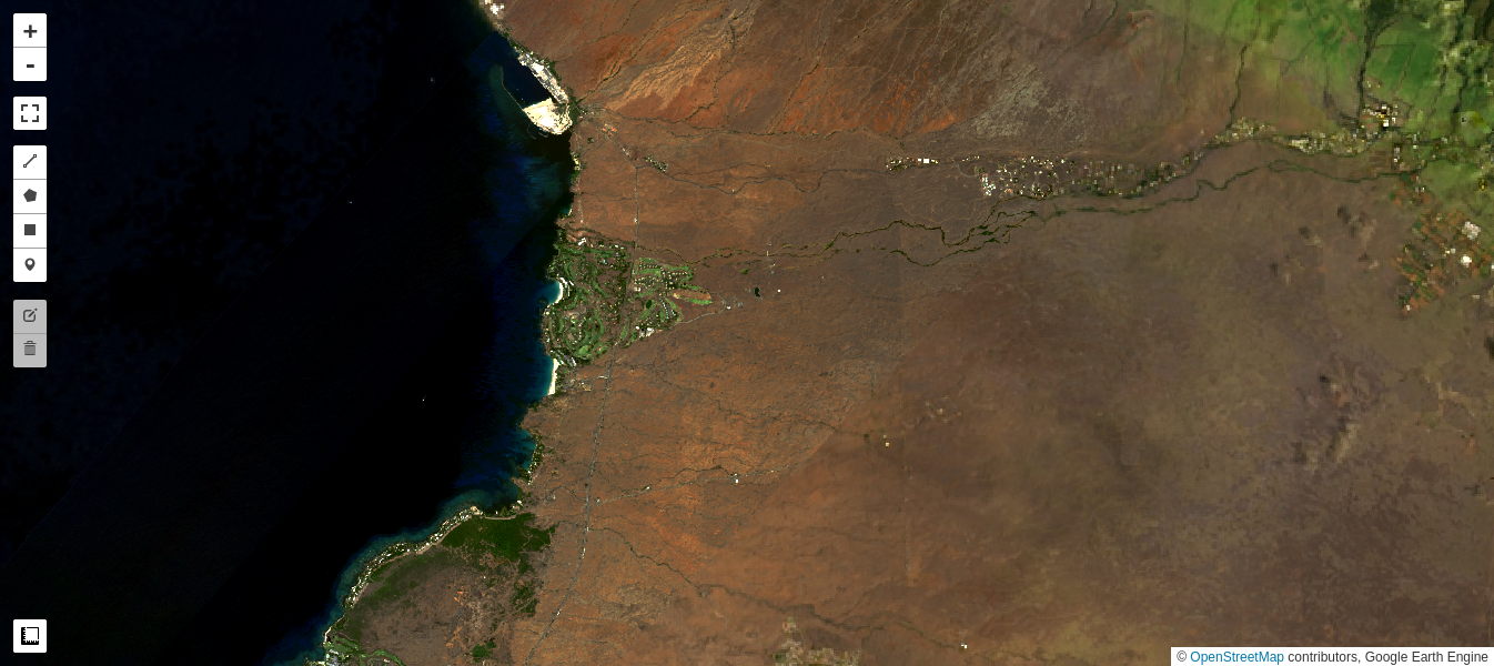
Results
Define a geemap.Map object, add layers, and display it. Until you zoom in really far, it's nearly impossible to tell where the Landsat image ends and the SkySat image begins.
lon, lat, zoom = -155.79584, 19.99866, 13
m = geemap.Map(center=[lat, lon], zoom=zoom)

vis_params_refl = {'min': 0, 'max': 0.25}
vis_params_dn = {'min': 0, 'max': 255}

m.add_layer(reference, vis_params_refl, 'Landsat-8 reference')
m.add_layer(skysat, vis_params_dn, 'SkySat source')
m.add_layer(result, vis_params_refl, 'SkySat matched')
m
Caveats
If there's anything anomalous in your image that's not in the reference image (or vice versa), like clouds, the CDF can end up skewed, and the histogram matching results might not look that good. Additionally, a little mis-registration between the source and target images is usually ok, since it is using the statistics of the whole region and doesn't really rely on a pixel-to-pixel correspondence.