Run me first
Run the following cell to initialize the API. The output will contain instructions on how to grant this notebook access to Earth Engine using your account.
import ee
# Trigger the authentication flow.
ee.Authenticate()

# Initialize the library.
ee.Initialize(project='my-project')
Datasets and Python modules
One dataset will be used in the tutorial:
- COPERNICUS/S1_GRD_FLOAT
- Sentinel-1 ground range detected images
The following cell imports some python modules which we will be using as we go along and enables inline graphics.
import matplotlib.pyplot as plt
import numpy as np
from scipy.stats import norm, gamma, f, chi2
import IPython.display as disp
%matplotlib inline
This cell carries over the chi square cumulative distribution function and the determinant of a Sentinel-1 image from Part 2.
def chi2cdf(chi2, df):
    """Calculates Chi square cumulative distribution function for
       df degrees of freedom using the built-in incomplete gamma
       function gammainc().
    """
    return ee.Image(chi2.divide(2)).gammainc(ee.Number(df).divide(2))

def det(im):
    """Calculates determinant of 2x2 diagonal covariance matrix."""
    return im.expression('b(0)*b(1)')
And to make use of interactive graphics, we import the folium package:
import folium
def add_ee_layer(self, ee_image_object, vis_params, name):
"""Adds Earth Engine layers to a folium map."""
map_id_dict = ee.Image(ee_image_object).getMapId(vis_params)
folium.raster_layers.TileLayer(
tiles = map_id_dict['tile_fetcher'].url_format,
attr = 'Map Data © <a href="https://earthengine.google.com/">Google Earth Engine</a>',
name = name,
overlay = True,
control = True).add_to(self)
# Add EE drawing method to folium.
folium.Map.add_ee_layer = add_ee_layer
Part 3. Multitemporal change detection
Continuing from Part 2, in which we discussed bitemporal change detection with Sentinel-1 images, we turn our attention to the multitemporal case. To get started, we obviously need ...
A time series
Here is a fairly interesting one: a region in South Yorkshire, England where, in November 2019, extensive flooding occurred along the River Don just north of the city of Doncaster.
geoJSON = {
  "type": "FeatureCollection",
  "features": [
    {
      "type": "Feature",
      "properties": {},
      "geometry": {
        "type": "Polygon",
        "coordinates": [
          [
            [
              -1.2998199462890625,
              53.48028242228504
            ],
            [
              -0.841827392578125,
              53.48028242228504
            ],
            [
              -0.841827392578125,
              53.6958933974518
            ],
            [
              -1.2998199462890625,
              53.6958933974518
            ],
            [
              -1.2998199462890625,
              53.48028242228504
            ]
          ]
        ]
      }
    }
  ]
}
coords = geoJSON['features'][0]['geometry']['coordinates']
aoi = ee.Geometry.Polygon(coords)
The image collection below covers the months of September, 2019 through January, 2020 at 6-day intervals:
im_coll = (ee.ImageCollection('COPERNICUS/S1_GRD_FLOAT')
           .filterBounds(aoi)
           .filterDate(ee.Date('2019-09-01'),ee.Date('2020-01-31'))
           .filter(ee.Filter.eq('orbitProperties_pass', 'DESCENDING'))
           .filter(ee.Filter.eq('relativeOrbitNumber_start', 154))
           .map(lambda img: img.set('date', ee.Date(img.date()).format('YYYYMMdd')))
           .sort('date'))

timestamplist = (im_coll.aggregate_array('date')
                 .map(lambda d: ee.String('T').cat(ee.String(d)))
                 .getInfo())
timestamplist
['T20190902',
 'T20190908',
 'T20190914',
 'T20190920',
 'T20190926',
 'T20191002',
 'T20191008',
 'T20191014',
 'T20191020',
 'T20191026',
 'T20191101',
 'T20191107',
 'T20191113',
 'T20191119',
 'T20191125',
 'T20191201',
 'T20191207',
 'T20191213',
 'T20191219',
 'T20191225',
 'T20191231',
 'T20200106',
 'T20200112',
 'T20200118',
 'T20200124',
 'T20200130']
It will turn out to be convenient to work with a list rather than a collection, so we'll convert the collection to a list and, while we're at it, clip the images to our AOI:
def clip_img(img):
    """Clips a list of images."""
    return ee.Image(img).clip(aoi)

im_list = im_coll.toList(im_coll.size())
im_list = ee.List(im_list.map(clip_img))

im_list.length().getInfo()
26
Here is an RGB composite of the VV bands for three images in early November, after conversion to decibels. Note that some changes, especially those due to flooding, already show up in this representation as colored pixels.
def selectvv(current):
    return ee.Image(current).select('VV')

vv_list = im_list.map(selectvv)

location = aoi.centroid().coordinates().getInfo()[::-1]
mp = folium.Map(location=location, zoom_start=11)
rgb_images = (ee.Image.rgb(vv_list.get(10), vv_list.get(11), vv_list.get(12))
              .log10().multiply(10))
mp.add_ee_layer(rgb_images, {'min': -20,'max': 0}, 'rgb composite')
mp.add_child(folium.LayerControl())
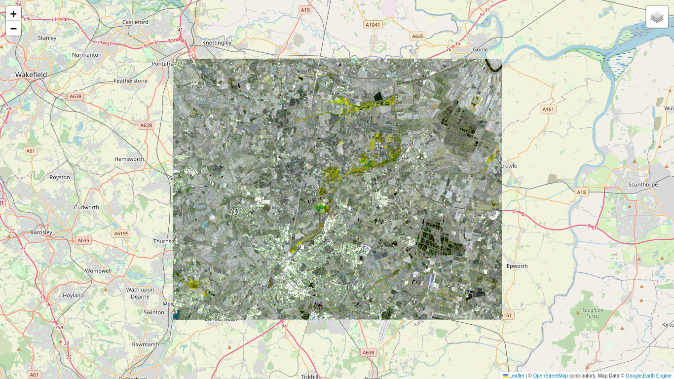
Now we have a series of 26 SAR images and, for whatever reason, would like to know where and when changes have taken place. A first reaction might be:
What's the problem? Just apply the bitemporal method we developed in Part 2 to each of the 25 time intervals.
Well, one problem is the rate of false positives. If the bitemporal tests are statistically independent, then the probability of not getting a false positive over a series of length \(k\) is the product of not getting one in each of the \(k-1\) intervals, i.e., \((1-\alpha)^{k-1}\) and the overall first kind error probability \(\alpha_T\) is its complement:
For our case, even with a small value of \(\alpha=0.01\), this gives a whopping 22.2% false positive rate:
alpha = 0.01
1-(1-alpha)**25
0.22217864060085335
Actually things are a bit worse. The bitemporal tests are manifestly not independent because consecutive tests have one image in common. The best one can say in this situation is
or \(\alpha_T \le 25\%\) for \(k=26\) and \(\alpha=0.01\) . If we wish to set a false positive rate of at most, say, 1% for the entire series, then each bitemporal test must have a significance level of \(\alpha=0.0004\) and a correspondingly large false negative rate \(\beta\). In other words many significant changes may be missed.
How to proceed? Perhaps by being a bit less ambitious at first and asking the simpler question: Were there any changes at all over the interval? If the answer is affirmative, we can worry about how many there were and when they occurred later. Let's formulate this question as ...
An omnibus test for change
We'll start again with the easier single polarization case. For the series of VV intensity images acquired at times \(t_1, t_2,\dots t_k\), our null hypothesis is that, at a given pixel position, there has been no change in the signal strengths \(a_i=\langle|S^{a_i}_{vv}|^2\rangle\) over the entire period, i.e.,
The alternative hypothesis is that there was at least one change (and possibly many) over the interval. For the more mathematically inclined this can be written succinctly as
which says: there exist indices \(i, j\) for which \(a_i\) is not equal to \(a_j\).
Again, the likelihood functions are products of gamma distributions:
and \(L_1\) is maximized for \(\hat a_i = s_i,\ i=1\dots k,\) while \(L_0\) is maximized for \(\hat a = {1\over k}\sum_i s_i\). So with a bit of simple algebra our likelihood ratio test statistic is
and is called an omnibus test statistic. Note that, for \(k=2\), we get the bitemporal LRT given by Eq. (2.10).
We can't expect to find an analytical expression for the probability distribution of this LRT statistic, so we will again invoke Wilks' Theorem and work with
According to Wilks, it should be approximately chi square distributed with \(k-1\) degrees of freedom under \(H_0\). (Why?)
The input cell below evaluates the test statistic Eq. (3.6) for a list of single polarization images. We prefer from now on to use as default the equivalent number of looks 4.4 that we discussed at the end of Part 1 rather than the actual number of looks \(m=5\), in the hope of getting a better agreement.
def omnibus(im_list, m = 4.4):
    """Calculates the omnibus test statistic, monovariate case."""
    def log(current):
        return ee.Image(current).log()

    im_list = ee.List(im_list)
    k = im_list.length()
    klogk = k.multiply(k.log())
    klogk = ee.Image.constant(klogk)
    sumlogs = ee.ImageCollection(im_list.map(log)).reduce(ee.Reducer.sum())
    logsum = ee.ImageCollection(im_list).reduce(ee.Reducer.sum()).log()
    return klogk.add(sumlogs).subtract(logsum.multiply(k)).multiply(-2*m)
Let's see if this test statistic does indeed follow the chi square distribution. First we define a small polygon aoi_sub over the Thorne Moors (on the eastern side of the AOI) for which we hope there are few significant changes.
geoJSON = {
  "type": "FeatureCollection",
  "features": [
    {
      "type": "Feature",
      "properties": {},
      "geometry": {
        "type": "Polygon",
        "coordinates": [
          [
            [
              -0.9207916259765625,
              53.63649628489509
            ],
            [
              -0.9225082397460938,
              53.62550271303527
            ],
            [
              -0.8892059326171875,
              53.61022911107819
            ],
            [
              -0.8737564086914062,
              53.627538775780984
            ],
            [
              -0.9207916259765625,
              53.63649628489509
            ]
          ]
        ]
      }
    }
  ]
}
coords = geoJSON['features'][0]['geometry']['coordinates']
aoi_sub = ee.Geometry.Polygon(coords)

location = aoi.centroid().coordinates().getInfo()[::-1]
mp = folium.Map(location=location, zoom_start=11)
mp.add_ee_layer(rgb_images.clip(aoi_sub), {'min': -20, 'max': 0}, 'aoi_sub rgb composite')
mp.add_child(folium.LayerControl())
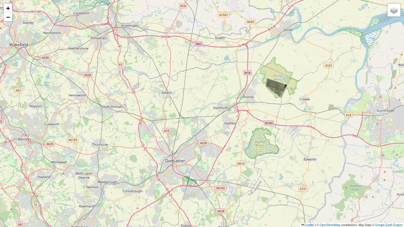
Here is a comparison for pixels in aoi_sub with the chi square distribution with \(k-1\) degrees of freedom. We choose the first 10 images in the series (\(k=10\)) because we expect fewer changes in September/October than over the complete sequence \(k=24\), which extends into January.
k = 10
hist = (omnibus(vv_list.slice(0,k))
        .reduceRegion(ee.Reducer.fixedHistogram(0, 40, 200), geometry=aoi_sub, scale=10)
        .get('constant')
        .getInfo())

a = np.array(hist)
x = a[:,0]
y = a[:,1]/np.sum(a[:,1])
plt.plot(x, y, '.', label='data')
plt.plot(x, chi2.pdf(x, k-1)/5, '-r', label='chi square')
plt.legend()
plt.grid()
plt.show()
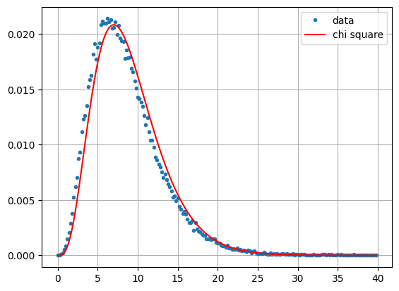
It appears that Wilks' Theorem is again a fairly good approximation. So why not generate a change map for the full series? The good news is that we now have the overall false positive probability \(\alpha\) under control. Here we set it to \(\alpha=0.01\).
# The change map for alpha = 0.01.
k = 26; alpha = 0.01
p_value = ee.Image.constant(1).subtract(chi2cdf(omnibus(vv_list), k-1))
c_map = p_value.multiply(0).where(p_value.lt(alpha), 1)
# Make the no-change pixels transparent.
c_map = c_map.updateMask(c_map.gt(0))
# Overlay onto the folium map.
location = aoi.centroid().coordinates().getInfo()[::-1]
mp = folium.Map(location=location, zoom_start=11)
mp.add_ee_layer(c_map, {'min': 0,'max': 1, 'palette': ['black', 'red']}, 'change map')
mp.add_child(folium.LayerControl())
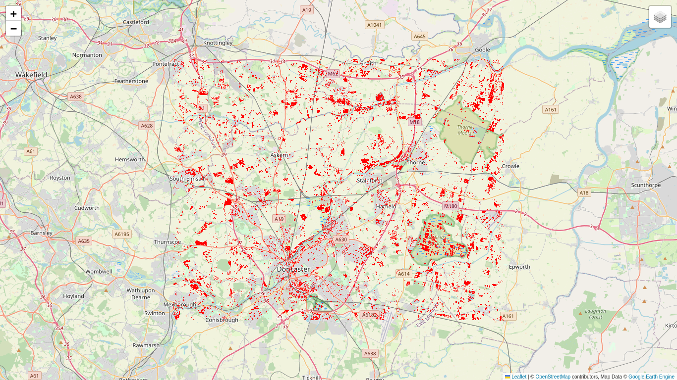
So plenty of changes, but hard to interpret considering the time span. Although we can see where changes took place, we know neither when they occurred nor their multiplicity. Also there is a matter that we have glossed over up until now, and that is ...
A question of scale
The number of looks plays an important role in all of the formulae that we have discussed so far, and for the Sentinel-1 ground range detected imagery we first used \(m=5\) and now the ENL \(=4.4\). When we display a change map interactively, the zoom factor determines the image pyramid level at which the GEE servers perform the required calculations and pass the result to the folium map client. If the calculations are not at the nominal scale of 10m then the number of looks is effectively larger than the ENL due to the averaging involved in constructing higher pyramid levels. The effect can be seen in the output cell above: the number of change pixels seems to decrease when we zoom out. There is no problem when we export our results to GEE assets, to Google Drive or to Cloud storage, since we can simply choose the correct nominal scale for export.
In order to see the changes correctly at all zoom levels, we can force GEE to work at the nominal scale by reprojecting before displaying on the map (use with caution):
c_map_10m = c_map.reproject(c_map.projection().crs(), scale=10)
mp = folium.Map(location=location, zoom_start=11)
mp.add_ee_layer(c_map, {'min': 0, 'max': 1, 'palette': ['black', 'red']}, 'Change map')
mp.add_ee_layer(c_map_10m, {'min': 0, 'max': 1, 'palette': ['black', 'blue']}, 'Change map (10m)')

mp.add_child(folium.LayerControl())
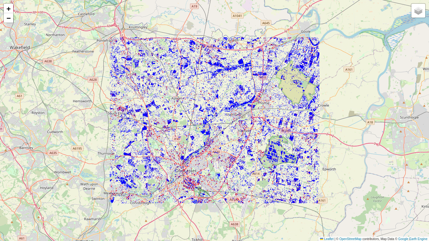
You will notice in the output cell above that the calculation at nominal scale (the blue pixels) now takes considerably longer to complete. Also some red pixels are not completely covered by blue ones. Those changes are a spurious result of the falsified number of looks. Nevertheless for quick previewing purposes we might prefer to do without the reprojection.
A sequential omnibus test
Recalling the last remark at the end of Part 2, let's now guess the omnibus LRT for the dual polarization case. From Eq. (3.5), replacing \(s_i \to|c_i|\), \(\ \sum s_i \to |\sum c_i|\ \) and \(k^k \to k^{2k}\), we get
This is in fact a special case of a more general omnibus test statistic
which holds for \(p\times p\) polarimetric covariance matrix images, for example for the full dual pol matrix Eq. (1.5) or for full \(3\times 3\) quad pol matrices (\(p=3\)), but also for diagonal \(2\times 2\) and \(3\times 3\) matrices.
Which brings us to the heart of this Tutorial. We will now decompose Eq. (3.7) into a product of independent likelihood ratio tests which will enable us to determine when changes occurred at each pixel location. Then we'll code a complete multitemporal change detection algorithm on the GEE Python API.
Single polarization
Rather than make a formal derivation, we will illustrate the decomposition on a series of \(k=5\) single polarization (VV) measurements. The omnibus test Eq. (3.5) for any change over the series from \(t_1\) to \(t_5\) is
If we accept the null hypothesis \(a_1=a_2=a_3=a_4=a_5\) we're done and can move on to the next pixel (figuratively of course, since this stuff is all done in parallel). But suppose we have rejected the null hypothesis, i.e., there was a least one significant change. In order to find it (or them), we begin by testing the first of the four intervals. That's just the bitemporal test from Part 2, but let's call it \(R_2\) rather than \(Q_2\),
Suppose we conclude no change, that is, \(a_1=a_2\). Now we don't do just another bitemporal test on the second interval. Instead we test the hypothesis
So the alternative hypothesis is: There was no change in the first interval and there was a change in the second interval. The LRT is easy to derive, but let's go through it anyway.
And, taking the ratio \(L_0/L_1\)of the maximum likelihoods,
Not too hard to guess that, if we accept \(H_0\) again, we go on to test
with LRT statistic
and so on to \(R_5\) and the end of the time series.
Now for the cool part (try it out yourself):
So, generalizing to a series of length \(k\):
The omnibus test statistic \(Q_k\) may be factored into the product of LRT's \(R_j\) which test for homogeneity in the measured reflectance signal up to and including time \(t_j\), assuming homogeneity up to time \(t_{j-1}\):
Moreover the test statistics \(R_j\) are stochastically independent under \(H_0\). This can be shown analytically, see Conradsen et al. (2016) or P. 405 in my textbook, but we'll show it here empirically by sampling the test statistics \(R_j\) in the region aoi_sub and examining the correlation matrix.
def sample_vv_imgs(j):
    """Samples the test statistics Rj in the region aoi_sub."""
    j = ee.Number(j)
    # Get the factors in the expression for Rj.
    sj = vv_list.get(j.subtract(1))
    jfact = j.pow(j).divide(j.subtract(1).pow(j.subtract(1)))
    sumj = ee.ImageCollection(vv_list.slice(0, j)).reduce(ee.Reducer.sum())
    sumjm1 = ee.ImageCollection(vv_list.slice(0, j.subtract(1))).reduce(ee.Reducer.sum())
    # Put them together.
    Rj = sumjm1.pow(j.subtract(1)).multiply(sj).multiply(jfact).divide(sumj.pow(j)).pow(5)
    # Sample Rj.
    sample = (Rj.sample(region=aoi_sub, scale=10, numPixels=1000, seed=123)
              .aggregate_array('VV_sum'))
    return sample

# Sample the first few list indices.
samples = ee.List.sequence(2, 8).map(sample_vv_imgs)

# Calculate and display the correlation matrix.
np.set_printoptions(precision=2, suppress=True)
print(np.corrcoef(samples.getInfo()))
[[ 1.    0.   -0.01 -0.04  0.03  0.06  0.02]
 [ 0.    1.    0.04 -0.01 -0.02  0.02  0.02]
 [-0.01  0.04  1.   -0.04  0.02 -0.02  0.04]
 [-0.04 -0.01 -0.04  1.   -0.04  0.01  0.03]
 [ 0.03 -0.02  0.02 -0.04  1.    0.08 -0.01]
 [ 0.06  0.02 -0.02  0.01  0.08  1.    0.  ]
 [ 0.02  0.02  0.04  0.03 -0.01  0.    1.  ]]
The off-diagonal elements are mostly small. The not-so-small values can be attributed to sampling error or to the presence of some change pixels in the samples.
Dual polarization and an algorithm
With our substitution trick, we can now write down the sequential test for the dual polarization (bivariate) image time series. From Eq. (3.8) we get
And of course we have again to use Wilks' Theorem to get the P values, so we work with
and
The statistic \(-2\log R_j\) is approximately chi square distributed with two degrees of freedom. Similarly \(-2\log Q_k\) is approximately chi square distributed with \(2(k-1)\) degrees of freedom. Readers should satisfy themselves that these numbers are indeed the correct, taking into account that each measurement \(c_i\) has two free parameters \(|S^a_{vv}|^2\) and \(|S^b_{vh}|^2\), see Eq. (2.13).
Now for the algorithm:
The sequential omnibus change detection algorithm
With a time series of \(k\) SAR images \((c_1,c_2,\dots,c_k)\),
- Set \(\ell = k\).
- Set \(s = (c_{k-\ell+1}, \dots c_k)\).
- Perform the omnibus test \(Q_\ell\) for any changes change over \(s\).
- If no significant changes are found, stop.
- Successively test series \(s\) with \(R_2, R_3, \dots\) until the first significant change is met for \(R_j\).
- Set \(\ell = k-j+1\) and go to 2.
| Table 3.1 | ||||||
|---|---|---|---|---|---|---|
| \(\ell\) | \(c_1\) | \(c_2\) | \(c_3\) | \(c_4\) | \(c_5\) | |
| 5 | \(R^5_2\) | \(R^5_3\) | \(R^5_4\) | \(R^5_5\) | \(Q_5\) | |
| 4 | \(R^4_2\) | \(R^4_3\) | \(R^4_4\) | \(Q_4\) | ||
| 3 | \(R^3_2\) | \(R^3_3\) | \(Q_3\) | |||
| 2 | \(R^2_2\) | \(Q_2\) |
Thus if a change is found, the series is truncated up to the point of change and the testing procedure is repeated for the rest of the series. Take for example a series of \(k=5\) images. (See Table 3.1 where, to avoid ambiguity, we add superscript \(\ell\) to each \(R_j\) test). Suppose there is one change in the second interval only. Then the test sequence is (the asterisk means \(H_0\) is rejected)
If there are changes in the second and last intervals,
and if there are significant changes in all four intervals,
The approach taken in the coding of this algorithm is to pre-calculate P values for all of the \(Q_\ell / R_j\) tests and then, in a second pass, to filter them to determine the points of change.
Pre-calculating the P value array
The following code cell performs map operations on the indices \(\ell\) and \(j\), returning an array of P values for all possible LRT statistics. For example again for \(k=5\), the code calculates the P values for each \(R_j\) entry in Table 3.1 as a list of lists. Before calculating each row, the time series \(c_1, c_2,c_3,c_4, c_5\) is sliced from \(k-\ell+1\) to \(k\). The last entry in each row is simply the product of the other entries, \(Q_\ell =\prod_{j=2}^\ell R_j.\)
The program actually operates on the logarithms of the test statistics, Equations (3.10).
def log_det_sum(im_list, j):
    """Returns log of determinant of the sum of the first j images in im_list."""
    im_ist = ee.List(im_list)
    sumj = ee.ImageCollection(im_list.slice(0, j)).reduce(ee.Reducer.sum())
    return ee.Image(det(sumj)).log()

def log_det(im_list, j):
    """Returns log of the determinant of the jth image in im_list."""
    im = ee.Image(ee.List(im_list).get(j.subtract(1)))
    return ee.Image(det(im)).log()

def pval(im_list, j, m=4.4):
    """Calculates -2logRj for im_list and returns P value and -2logRj."""
    im_list = ee.List(im_list)
    j = ee.Number(j)
    m2logRj = (log_det_sum(im_list, j.subtract(1))
               .multiply(j.subtract(1))
               .add(log_det(im_list, j))
               .add(ee.Number(2).multiply(j).multiply(j.log()))
               .subtract(ee.Number(2).multiply(j.subtract(1))
               .multiply(j.subtract(1).log()))
               .subtract(log_det_sum(im_list,j).multiply(j))
               .multiply(-2).multiply(m))
    pv = ee.Image.constant(1).subtract(chi2cdf(m2logRj, 2))
    return (pv, m2logRj)

def p_values(im_list):
    """Pre-calculates the P-value array for a list of images."""
    im_list = ee.List(im_list)
    k = im_list.length()

    def ells_map(ell):
        """Arranges calculation of pval for combinations of k and j."""
        ell = ee.Number(ell)
        # Slice the series from k-l+1 to k (image indices start from 0).
        im_list_ell = im_list.slice(k.subtract(ell), k)

        def js_map(j):
            """Applies pval calculation for combinations of k and j."""
            j = ee.Number(j)
            pv1, m2logRj1 = pval(im_list_ell, j)
            return ee.Feature(None, {'pv': pv1, 'm2logRj': m2logRj1})

        # Map over j=2,3,...,l.
        js = ee.List.sequence(2, ell)
        pv_m2logRj = ee.FeatureCollection(js.map(js_map))

        # Calculate m2logQl from collection of m2logRj images.
        m2logQl = ee.ImageCollection(pv_m2logRj.aggregate_array('m2logRj')).sum()
        pvQl = ee.Image.constant(1).subtract(chi2cdf(m2logQl, ell.subtract(1).multiply(2)))
        pvs = ee.List(pv_m2logRj.aggregate_array('pv')).add(pvQl)
        return pvs

    # Map over l = k to 2.
    ells = ee.List.sequence(k, 2, -1)
    pv_arr = ells.map(ells_map)

    # Return the P value array ell = k,...,2, j = 2,...,l.
    return pv_arr
Filtering the P values
| Table 3.2 | ||||||
|---|---|---|---|---|---|---|
| \(i\ \) / \(j\) | 1 | 2 | 3 | 4 | ||
| 1 | \(P_2\) | \(P_3\) | \(P_4\) | \(P_5\) | \(P_{Q5}\) | |
| 2 | \(P_2\) | \(P_3\) | \(P_4\) | \(P_{Q4}\) | ||
| 3 | \(P_2\) | \(P_3\) | \(P_{Q3}\) | |||
| 4 | \(P_2\) | \(P_{Q2}\) |
The pre-calculated P values in pv_arr (shown schematically in Table 3.2 for \(k=5\)) are then scanned in nested iterations over indices \(i\) and \(j\) to determine the following thematic change maps:
- cmap: the interval of the most recent change, one band, byte values \(\in [0,k-1]\),
- smap: the interval of the first change, one band, byte values \(\in [0,k-1]\),
- fmap: the number of changes, one band, byte values \(\in [0,k-1]\),
- bmap: the changes in each interval, \(\ k-1\) bands, byte values \(\in [0,1]\)).
A boolean variable median is included in the code. Its purpose is to reduce the salt-and-pepper effect in no-change regions, which is at least partly a consequence of the uniform distribution of the P values under \(H_0\) (see the section A note on P values in Part 2). If median is True, the P values for each \(Q_\ell\) statistic are passed through a \(5\times 5\) median filter before being compared with the significance threshold. This is not statistically kosher but probably justifiable if one is only interested in large homogeneous changes, for example flood inundations or deforestation.
Here is the code:
def filter_j(current, prev):
    """Calculates change maps; iterates over j indices of pv_arr."""
    pv = ee.Image(current)
    prev = ee.Dictionary(prev)
    pvQ = ee.Image(prev.get('pvQ'))
    i = ee.Number(prev.get('i'))
    cmap = ee.Image(prev.get('cmap'))
    smap = ee.Image(prev.get('smap'))
    fmap = ee.Image(prev.get('fmap'))
    bmap = ee.Image(prev.get('bmap'))
    alpha = ee.Image(prev.get('alpha'))
    j = ee.Number(prev.get('j'))
    cmapj = cmap.multiply(0).add(i.add(j).subtract(1))
    # Check      Rj?            Ql?                  Row i?
    tst = pv.lt(alpha).And(pvQ.lt(alpha)).And(cmap.eq(i.subtract(1)))
    # Then update cmap...
    cmap = cmap.where(tst, cmapj)
    # ...and fmap...
    fmap = fmap.where(tst, fmap.add(1))
    # ...and smap only if in first row.
    smap = ee.Algorithms.If(i.eq(1), smap.where(tst, cmapj), smap)
    # Create bmap band and add it to bmap image.
    idx = i.add(j).subtract(2)
    tmp = bmap.select(idx)
    bname = bmap.bandNames().get(idx)
    tmp = tmp.where(tst, 1)
    tmp = tmp.rename([bname])
    bmap = bmap.addBands(tmp, [bname], True)
    return ee.Dictionary({'i': i, 'j': j.add(1), 'alpha': alpha, 'pvQ': pvQ,
                          'cmap': cmap, 'smap': smap, 'fmap': fmap, 'bmap':bmap})

def filter_i(current, prev):
    """Arranges calculation of change maps; iterates over row-indices of pv_arr."""
    current = ee.List(current)
    pvs = current.slice(0, -1 )
    pvQ = ee.Image(current.get(-1))
    prev = ee.Dictionary(prev)
    i = ee.Number(prev.get('i'))
    alpha = ee.Image(prev.get('alpha'))
    median = prev.get('median')
    # Filter Ql p value if desired.
    pvQ = ee.Algorithms.If(median, pvQ.focalMedian(2.5), pvQ)
    cmap = prev.get('cmap')
    smap = prev.get('smap')
    fmap = prev.get('fmap')
    bmap = prev.get('bmap')
    first = ee.Dictionary({'i': i, 'j': 1, 'alpha': alpha ,'pvQ': pvQ,
                           'cmap': cmap, 'smap': smap, 'fmap': fmap, 'bmap': bmap})
    result = ee.Dictionary(ee.List(pvs).iterate(filter_j, first))
    return ee.Dictionary({'i': i.add(1), 'alpha': alpha, 'median': median,
                          'cmap': result.get('cmap'), 'smap': result.get('smap'),
                          'fmap': result.get('fmap'), 'bmap': result.get('bmap')})
The following function ties the two steps together:
def change_maps(im_list, median=False, alpha=0.01):
    """Calculates thematic change maps."""
    k = im_list.length()
    # Pre-calculate the P value array.
    pv_arr = ee.List(p_values(im_list))
    # Filter P values for change maps.
    cmap = ee.Image(im_list.get(0)).select(0).multiply(0)
    bmap = ee.Image.constant(ee.List.repeat(0, k.subtract(1))).add(cmap)
    alpha = ee.Image.constant(alpha)
    first = ee.Dictionary({'i': 1, 'alpha': alpha, 'median': median,
                           'cmap': cmap, 'smap': cmap, 'fmap': cmap, 'bmap': bmap})
    return ee.Dictionary(pv_arr.iterate(filter_i, first))
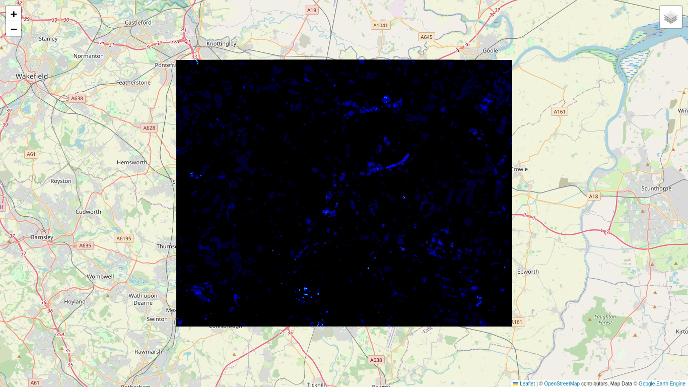
And now we run the algorithm and display the color-coded change maps: cmap, smap (blue early, red late) and fmap (blue few, red many):
result = change_maps(im_list, median=True, alpha=0.05)

# Extract the change maps and display.
cmap = ee.Image(result.get('cmap'))
smap = ee.Image(result.get('smap'))
fmap = ee.Image(result.get('fmap'))
location = aoi.centroid().coordinates().getInfo()[::-1]
palette = ['black', 'blue', 'cyan', 'yellow', 'red']
mp = folium.Map(location=location, zoom_start=11)
mp.add_ee_layer(cmap, {'min': 0, 'max': 25, 'palette': palette}, 'cmap')
mp.add_ee_layer(smap, {'min': 0, 'max': 25, 'palette': palette}, 'smap')
mp.add_ee_layer(fmap, {'min': 0, 'max': 25, 'palette': palette}, 'fmap')
mp.add_child(folium.LayerControl())
Post-processing: The Loewner order
The above change maps are still difficult to interpret. But what about bmap, the map of changes detected in each interval? Before we look at them it makes sense to include the direction of change, i.e., the Loewner order, see Part 2. In the event of significant change at time \(j\), we can simply determine the positive or negative definiteness (or indefiniteness) of the difference between consecutive covariance matrix pixels
to get the change direction. But we can do better. Instead of subtracting the value for the preceding image, \(c_{j-1}\), we can subtract the average over all values up to and including time \(j-1\) for which no change has been signalled. For example for \(k=5\), suppose there are significant changes in the first and fourth (last) interval. Then to get their directions we examine the differences
The running averages can be conveniently determined with the so-called provisional means algorithm. The average \(\bar c_i\) of the first \(i\) images is calculated recursively as
The function dmap_iter below is iterated over the bands of bmap, replacing the values for changed pixels with
- 1 for positive definite differences,
- 2 for negative definite differences,
- 3 for indefinite differences.
def dmap_iter(current, prev):
    """Reclassifies values in directional change maps."""
    prev = ee.Dictionary(prev)
    j = ee.Number(prev.get('j'))
    image = ee.Image(current)
    avimg = ee.Image(prev.get('avimg'))
    diff = image.subtract(avimg)
    # Get positive/negative definiteness.
    posd = ee.Image(diff.select(0).gt(0).And(det(diff).gt(0)))
    negd = ee.Image(diff.select(0).lt(0).And(det(diff).gt(0)))
    bmap = ee.Image(prev.get('bmap'))
    bmapj = bmap.select(j)
    dmap = ee.Image.constant(ee.List.sequence(1, 3))
    bmapj = bmapj.where(bmapj, dmap.select(2))
    bmapj = bmapj.where(bmapj.And(posd), dmap.select(0))
    bmapj = bmapj.where(bmapj.And(negd), dmap.select(1))
    bmap = bmap.addBands(bmapj, overwrite=True)
    # Update avimg with provisional means.
    i = ee.Image(prev.get('i')).add(1)
    avimg = avimg.add(image.subtract(avimg).divide(i))
    # Reset avimg to current image and set i=1 if change occurred.
    avimg = avimg.where(bmapj, image)
    i = i.where(bmapj, 1)
    return ee.Dictionary({'avimg': avimg, 'bmap': bmap, 'j': j.add(1), 'i': i})
We only have to modify the change_maps function to include the change direction in the bmap image:
def change_maps(im_list, median=False, alpha=0.01):
    """Calculates thematic change maps."""
    k = im_list.length()
    # Pre-calculate the P value array.
    pv_arr = ee.List(p_values(im_list))
    # Filter P values for change maps.
    cmap = ee.Image(im_list.get(0)).select(0).multiply(0)
    bmap = ee.Image.constant(ee.List.repeat(0,k.subtract(1))).add(cmap)
    alpha = ee.Image.constant(alpha)
    first = ee.Dictionary({'i': 1, 'alpha': alpha, 'median': median,
                           'cmap': cmap, 'smap': cmap, 'fmap': cmap, 'bmap': bmap})
    result = ee.Dictionary(pv_arr.iterate(filter_i, first))
    # Post-process bmap for change direction.
    bmap =  ee.Image(result.get('bmap'))
    avimg = ee.Image(im_list.get(0))
    j = ee.Number(0)
    i = ee.Image.constant(1)
    first = ee.Dictionary({'avimg': avimg, 'bmap': bmap, 'j': j, 'i': i})
    dmap = ee.Dictionary(im_list.slice(1).iterate(dmap_iter, first)).get('bmap')
    return ee.Dictionary(result.set('bmap', dmap))
Because of the long delays when the zoom level is changed, it is a lot more convenient to export the change maps to GEE Assets and then examine them, either here in Colab or in the Code Editor. This also means the maps will be shown at the correct scale, irrespective of the zoom level. Here I export all of the change maps as a single image.
# Run the algorithm with median filter and at 1% significance.
result = ee.Dictionary(change_maps(im_list, median=True, alpha=0.01))
# Extract the change maps and export to assets.
cmap = ee.Image(result.get('cmap'))
smap = ee.Image(result.get('smap'))
fmap = ee.Image(result.get('fmap'))
bmap = ee.Image(result.get('bmap'))
cmaps = ee.Image.cat(cmap, smap, fmap, bmap).rename(['cmap', 'smap', 'fmap']+timestamplist[1:])

# EDIT THE ASSET PATH TO POINT TO YOUR ACCOUNT.
assetId = 'users/YOUR_USER_NAME/cmaps'

assexport = ee.batch.Export.image.toAsset(cmaps,
                                          description='assetExportTask',
                                          assetId=assetId, scale=10, maxPixels=1e9)

# UNCOMMENT THIS TO EXPORT THE MAP TO YOUR ACCOUNT.
#assexport.start()
The asset cmaps is shared so we can all access it:
cmaps = ee.Image('projects/earthengine-community/tutorials/detecting-changes-in-sentinel-1-imagery-pt-3/cmaps')
cmaps = cmaps.updateMask(cmaps.gt(0))

location = aoi.centroid().coordinates().getInfo()[::-1]
palette = ['black', 'red', 'cyan', 'yellow']
mp = folium.Map(location=location, zoom_start=13)

mp.add_ee_layer(cmaps.select('T20191107'), {'min': 0,'max': 3, 'palette': palette}, 'T20191107')
mp.add_ee_layer(cmaps.select('T20191113'), {'min': 0,'max': 3, 'palette': palette}, 'T20191113')
mp.add_ee_layer(cmaps.select('T20191119'), {'min': 0,'max': 3, 'palette': palette}, 'T20191119')
mp.add_ee_layer(cmaps.select('T20191125'), {'min': 0,'max': 3, 'palette': palette}, 'T20191125')
mp.add_ee_layer(cmaps.select('T20191201'), {'min': 0,'max': 3, 'palette': palette}, 'T20191201')
mp.add_ee_layer(cmaps.select('T20191207'), {'min': 0,'max': 3, 'palette': palette}, 'T20191207')

mp.add_child(folium.LayerControl())
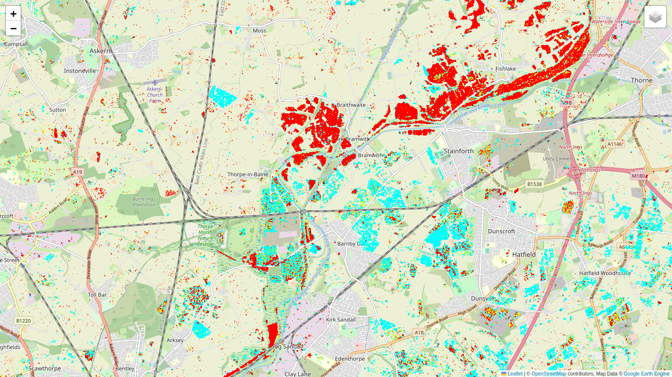
Now interpretation is somewhat easier. The negative definite (cyan) changes which appear between Nov. 7 and Nov. 13 correspond to decreases in intensity of VV and VH reflectance and are due to wide-spread flooding. The positive definite changes (red), which gradually overlay the flooded areas in subsequent intervals, correspond to receding flood waters.
Outlook
Without reliable ground truth we can't really claim that change maps of the kind we have just generated will be helpful for flood damage assessment or control, but their potential usefulness is quite obvious. In the next and final part of the Tutorial we will have a look at some more (possible) applications of sequential change detection with SAR imagery using GEE.
 Run in Google Colab
 View source on GitHub