In general, media has a lagged effect on KPI where the effects taper off over time. To model this lagged effect we transform the media execution of a given channel through the Adstock function:
where:
\(w(s; \alpha) \) is a non-negative weight function,
\(x_s \geq 0\) is media execution at time \(s\),
\(\alpha\ \in\ [0, 1]\) is the decay parameter,
\(L\) is the maximum lag duration.
Meridian provides two decay curves, geometric and binomial. The rate
at which the media effect taper off occurs is governed by the choice of function
along with the learned parameter alpha. The adstock_decay_spec parameter
of ModelSpec defines which function, or combination of functions, are used.
For example, to use binomial decay all channels, you can use:
from meridian.model import spec

model_spec = spec.ModelSpec(
  adstock_decay_spec='binomial'
)
Whereas to use binomial, geometric, and binomial for three channels named
"Channel0", "Channel1", and "Channel2", respectively, you can specify:
from meridian.model import spec

model_spec = spec.ModelSpec(
  adstock_decay_spec=dict(
    Channel0='binomial',
    Channel1='geometric',
    Channel2='binomial',
  )
)
In general, we recommend using binomial decay when you think a significant proportion of a media channel's lagged effects persist into the latter half of the effect window. Otherwise, we recommend using geometric decay.
These functions define weights \(w(s; \alpha)\) for the Adstock function. They are defined such that at time \(t\), the media execution at time \(t-s\) has weight \(w(s; \alpha) / \sum_{s\in{\{0, ..., L\}}}w(s; \alpha)\). For additional details on the Adstock function, see Media saturation and lagging.
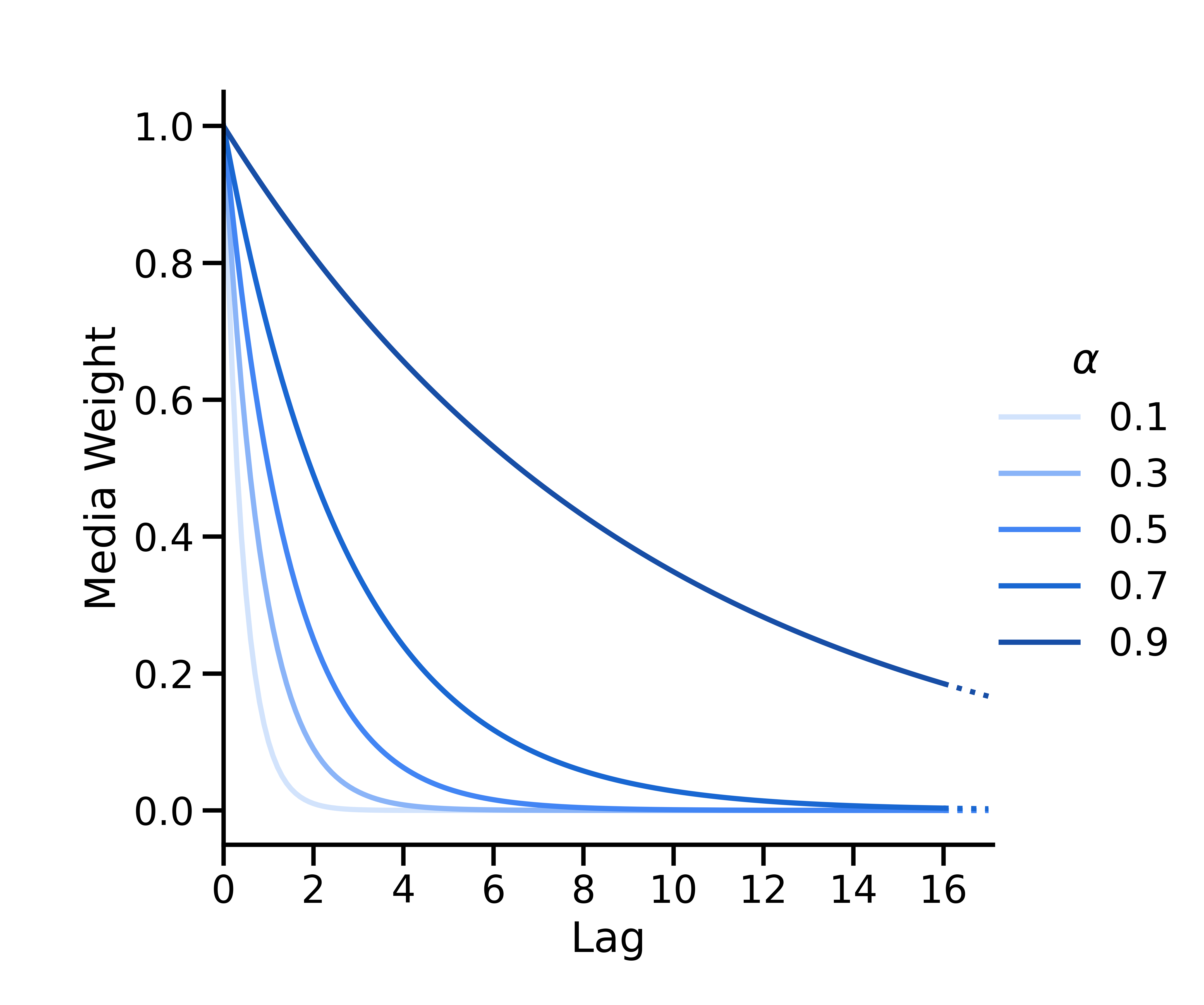
Geometric decay
Geometric decay is parameterized as \(w(s; \alpha) = \alpha^s\), where \(\alpha \in [0, 1] \) is the geometric parameter denoting the decay rate and \(s\) is the lag. At time \(t\), the media execution at time \(t-s\) has weight \(w(s; \alpha) = \alpha^s\), which is then normalized so that all weights sum to one.
Binomial decay
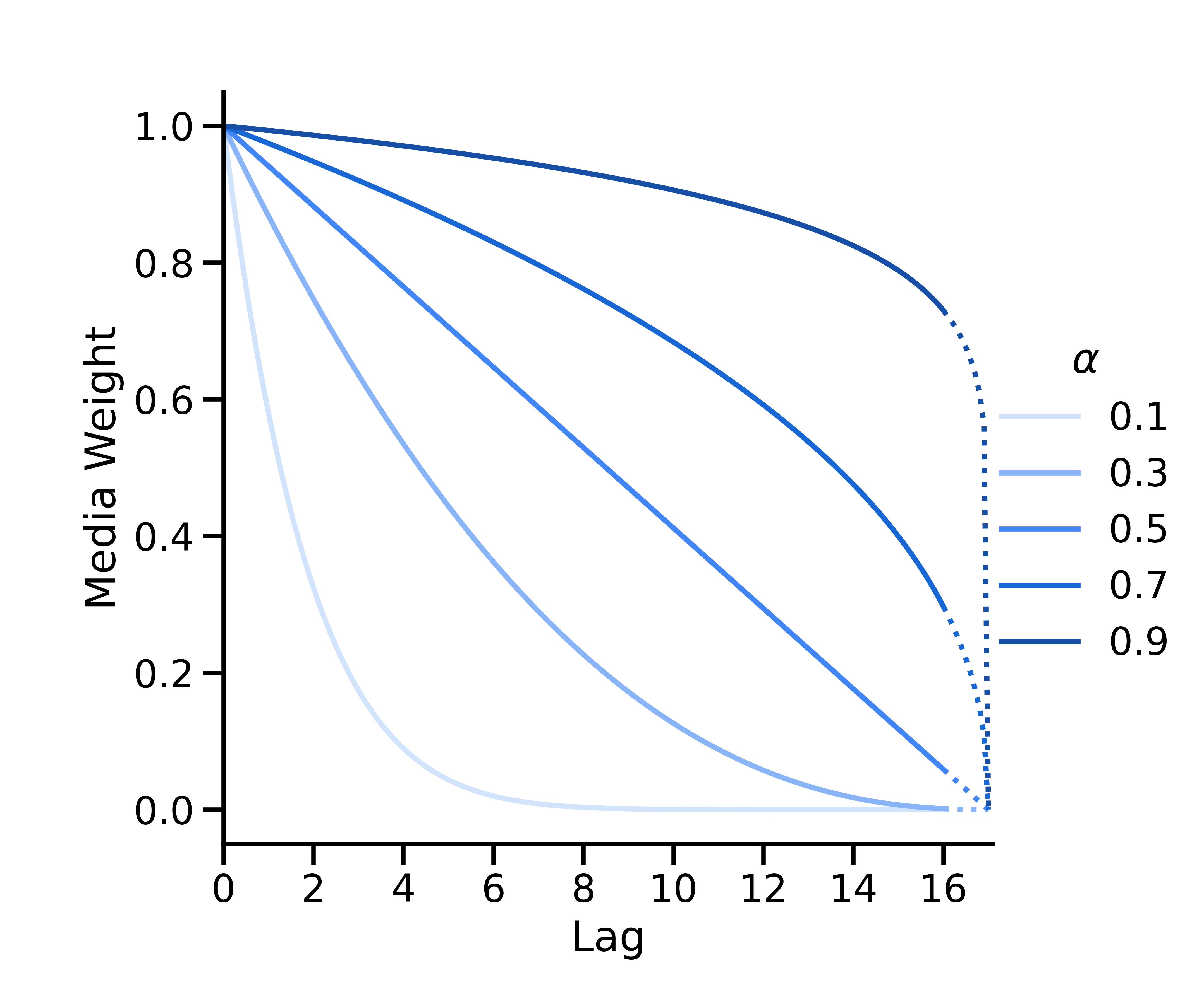
Binomial decay is parameterized as
where \(L\) is the max lag (the max_lag parameter of ModelSpec). The
mapping \(\alpha_*=\frac{1}{\alpha} - 1\) is used to map values of
\(\alpha\) from \([0, 1]\) to \([0, \infty)\).
The binomial curve is convex if \(\alpha < 0.5\), linear if \(\alpha = 0.5\) and concave if \(\alpha > 0.5\). It is defined such that its x-intercept is always at \(L + 1\).
Decide between geometric and binomial decay
We recommend selecting binomial decay when you think a channel has a significant proportion of effects in the latter half of the effects window. Otherwise, pick geometric decay.
The decay curve impacts the relative weights of lagged media. Increasing the
relative weight of later time periods necessarily decreases the relative
weight of earlier time periods. The binomial decay curve defines weights that
decay to zero more gradually than the geometric curve. Therefore, the binomial
decay curve encourages a larger proportion of a channel's total media effect to
happen in later time periods, whereas the geometric decay curve encourages a
larger proportion of a channel's total media effect to happen in earlier time
periods. The binomial decay curve is a good choice when using larger values of
max_lag because it is "stretched" to cover the effect window, since its
x-intercept is always at \(L + 1\). See
Set the max_lag parameter
for additional details.
It can be tempting to select the binomial decay curve for all channels due to
its ability to support larger max_lag values. However, keep in
mind that not all channels will be best modeled by the binomial decay curve,
which is best used when you think a channel has a significant proportion of
effects in the latter half of the effects window. Misapplication of the binomial
decay curve can result in an underestimation of short term effects.
| Function | Geometric | Binomial |
|---|---|---|
| Best For | Media with short-lived effects. | Media with effects that persist to the latter half of the effect window. |
| Curve Shape | Fast decay. | Can persist longer before decaying. |
| Max Lag Recommendation | 2-10 time periods. | 4-20 time periods. |
| Drawbacks | Vulnerable to long-term effect underestimation. | Vulnerable to short-term effect underestimation. |
Considerations for long term effects
If you expect long term effects that are not materializing in a model, some
combination of the binomial decay curve, modifying the prior on alpha, and
changing the max_lag can help. Use the prior curves from
MediaEffects.plot_adstock_decay
to see how max_lag, alpha prior, and decay function all interact with each
other. You can then fine tune these to align a model with your initial
assumptions about lagged effects. Modifying the prior and max_lag can be done
alongside or instead of selecting a particular decay function. We recommend
experimenting with different combinations to balance convergence, model fit and
effect window. See
Set the max_lag parameter
for additional details on selecting a value of max_lag.
The alpha prior
The default alpha prior in Meridian is \(U(0, 1)\), which is an uninformative prior for both geometric and binomial decay functions. If you have intuition about the rate at which the media effect tapers off for a particular channel, you can set a custom alpha prior on that channel to inform Meridian about your intuition.
For both geometric and binomial decay, there is a monotonic relationship between \(\alpha\) and the rate at which the media effect decays: smaller \(\alpha\) corresponds to faster decay and larger \(\alpha\) corresponds to shorter decay. Geometric and binomial functions both maximize short term effects when \(\alpha=0\), in which case there are no lagged effects, and maximize long term effects when \(\alpha=1\), in which case all media within the historical lagged window are weighted equally.
As a result, we recommend setting a prior on alpha with more of its mass near
zero to encourage faster decay and shorter term effects. For example, a
Beta(1, 3) distribution has more mass near zero compared to the default uniform
distribution. Conversely, we recommend setting a prior with more of its mass
near one to encourage slower decay and longer term effects. For example, a
Beta(3, 1) distribution has more mass near one compared to the default uniform
distribution. We recommend plotting prior distributions of both alpha and media
weights (using
MediaEffects.plot_adstock_decay)
to confirm custom prior distributions match your intuitions.
The binomial \(\alpha\) map
The mapping \(\alpha_*: [0, 1]\rightarrow[0, \infty) \) is performed because the binomial function decays for \(\alpha_* \in [0, \infty)\) while the geometric function decays for \(\alpha \in [0, 1]\). This mapping allows for priors defined on the interval \([0, 1]\) to be correctly translated to \([0, \infty)\) in the binomial case and retains model specification consistency with geometric decay, with low values of alpha implying fast decay and shorter term effects and higher values of alpha implying slow decay and longer term effects.
Advanced option: set a custom prior directly on \(\alpha_*\) when using binomial
Meridian uses a default prior of \(U(0, 1)\) on \(\alpha\) for both geometric and binomial functions. With binomial decay, a \(U(0, 1)\) prior on \(\alpha\) is equivalent to a Lomax(1, 1) prior on \(\alpha_*\):
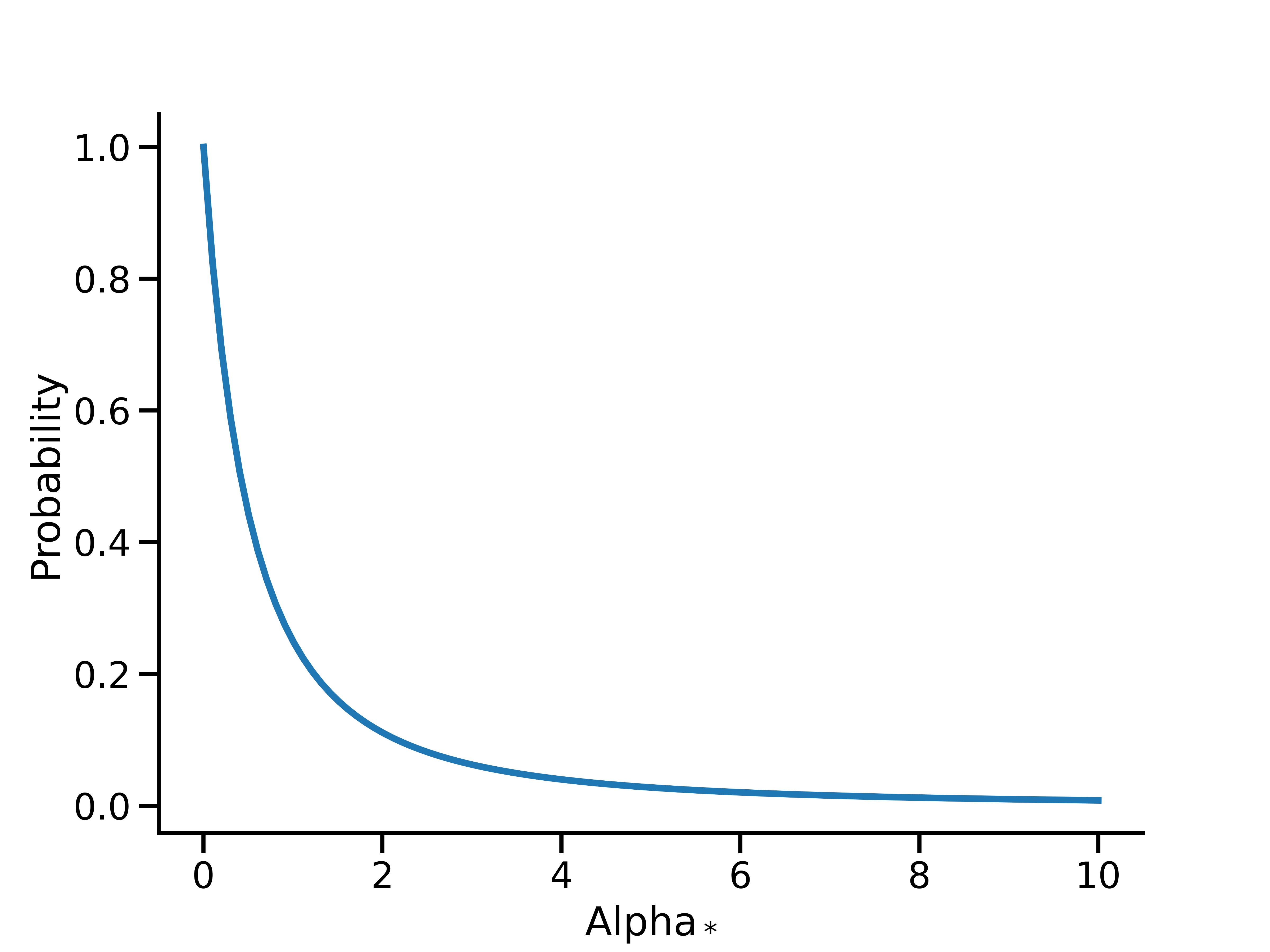
This remains a relatively uninformative prior to allow data to inform the decay rate with binomial decay.
Meridian expects custom \(\alpha\) priors to have support of \([0, 1]\) (for
example, a Beta distribution) which will then be mapped to the non-negative
real numbers with \(1/x-1\). If, however, you would like to be able to define
a prior on \(\alpha_*\) with support of \([0, \infty)\) you may do so and
then transform it with the inverse mapping \(\frac{1}{1+x}\). This mapping is
available through the helper method
adstock_hill.transform_non_negative_reals_distribution.
For example, to end up with a lognormal prior on \(\alpha_*\) with a mean of
0.5 and a variance of 0.5:
import tensorflow as tf

# Example: pick mu, sigma so that the mean, variance of alpha_* are both 0.5
mu = -tf.math.log(2.0) - 0.5 * tf.math.log(3.0)
sigma = tf.math.sqrt(tf.math.log(3.0))

alpha_star_prior = tfp.distributions.LogNormal(mu, sigma)  # prior on alpha_* for binomial
alpha_prior = adstock_hill.transform_non_negative_reals_distribution(alpha_star_prior)

prior = prior_distribution.PriorDistribution(
  alpha_m=alpha_prior
)

model_spec = spec.ModelSpec(
  prior=prior,
  adstock_decay_spec='binomial'
)
You may then also interrogate the alpha prior directly. For example, to view the probability density function on alpha:
import numpy as np
from matplotlib import pyplot as plt

x = np.linspace(0, 1, 100)
fig, ax = plt.subplots(figsize=(8, 6))
ax.plot(x, alpha_prior.prob(x), linewidth=3)
ax.set(xlabel='Alpha', ylabel='Probability')
plt.show()
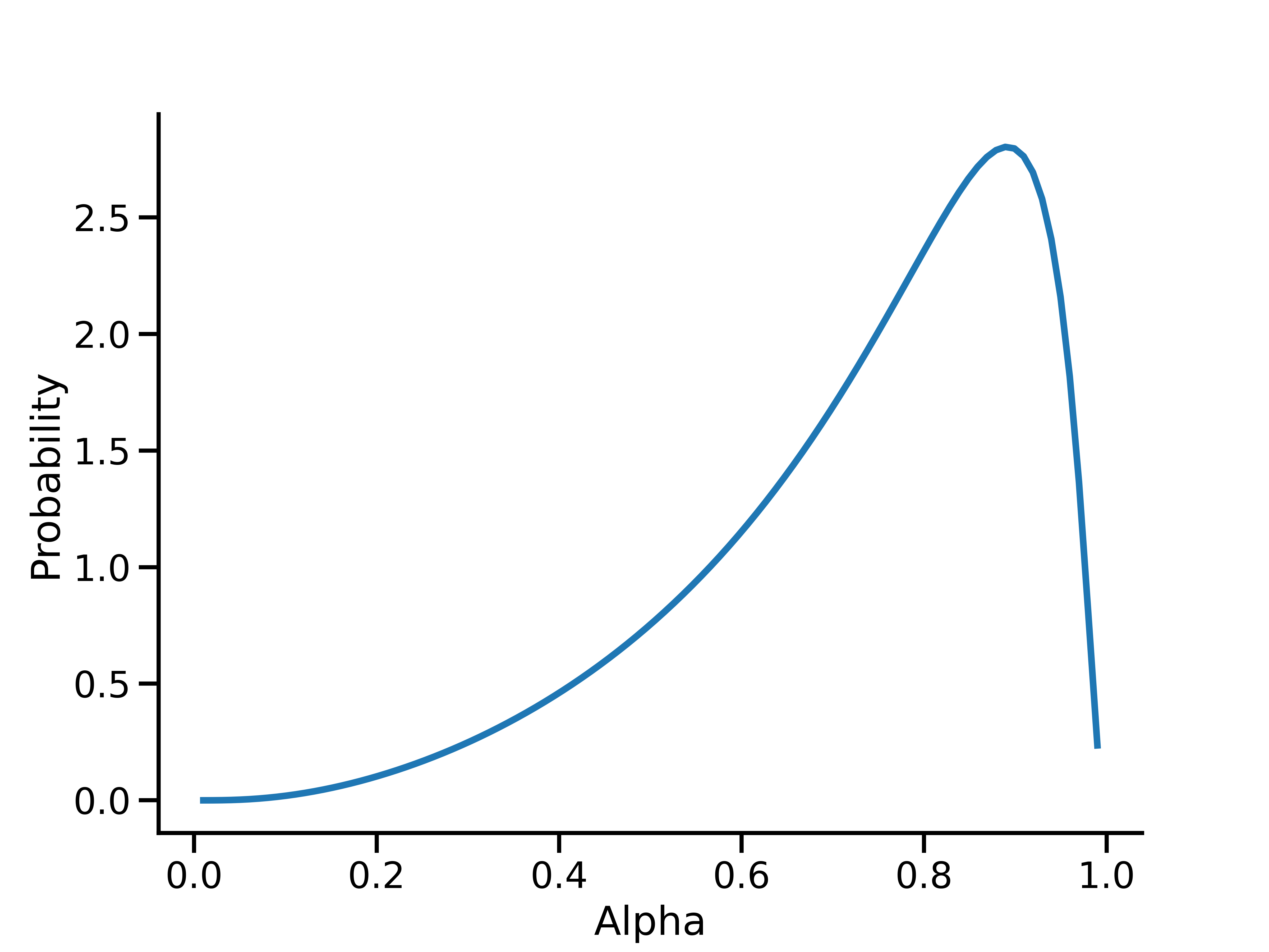
This plot shows the prior on \(\alpha\) that leads to a lognormal prior on \(\alpha_*\) with mean and variance of 0.5 and 0.5, respectively.