Scenario planning and future budget optimization

This section covers how to use Meridian for scenario planning, including how to incorporate data and assumptions about the future into budget optimization scenarios.

As part of future budget optimization, Meridian forecasts incremental outcome under a set of assumptions about the future. Meridian does not predict the future outcome value itself, only the incremental portion. More detail is provided in Why Meridian doesn't forecast outcome.

What is scenario planning?

Scenario planning is MMM analysis that can incorporate assumptions about the future. For post-modeling analysis such as ROI, response curves, and budget optimization, Meridian uses historical data to make default assumptions. Sometimes these assumptions are reasonable for future planning, but not always. New data can be incorporated into the analysis to modify the assumptions as needed.

The following are some ways future strategies may differ from historical.

• Cost per media unit: The cost per media unit on a channel may have changed or be expected to change. (See Coding Example 1 and Example 2)
• Revenue per KPI unit: The revenue per KPI (e.g. unit price or lifetime value) may have changed or be expected to change. (See Coding Example 3)
• Flighting Pattern: Your historical and future flighting patterns may not match. For example, you may have introduced a new media channel during the model training window. The historical flighting pattern of the new channel might contain zeros or show a "ramping up" trend that is not expected to continue. (See Coding Example 4)

Post-modeling analysis metrics

Scenario planning effects metric definitions but not parameter estimation. To illustrate these concepts, consider a hypothetical case where ordinary least squares is used to estimate the treatment effect of a drug where we hypothesize that the dosage in mg (X) linearly affects the outcome (Y) such as in the model,

\[ Y = \alpha + X \beta + \epsilon \ . \]

The treatment effect depends on the dosage coefficient $\beta$, which is a parameter estimated from an observed dataset. The treatment effect can have many possible metric definitions. For example, you could define the effect of a drug as the expected change in outcome caused by a 10 mg dose ($10 \beta$) or a 15 mg dose ($15 \beta$). You can estimate both treatment effect definitions using the same model and coefficient estimate $\hat{\beta}$.

In Meridian, the definition of post-modeling analysis metrics depends on certain data characteristics. For example, the ROI depends on a specified time range, set of geos, flighting pattern (relative distribution of media units across geos and time periods), total media units per channel, cost per media unit, and revenue per KPI. Other post-modeling analysis metrics include expected outcome, incremental outcome, marginal ROI, CPIK, response curves, and optimal budget allocation. By default, these metrics are defined using the input_data passed to Meridian; however, new_data can be provided to specify alternative metric definitions. A table indicating which of the data properties affect each metric's definition is provided in Table 1.

‡ Budget optimization uses the total media units per channel (in combination with the fixed flighting pattern and cost per media unit assumptions) to assign a default total budget (fixed budget optimization only) and channel-level budget constraints. If these settings are overridden using the budget andpct_of_spend arguments of BudgetOptimizer.optimize, then the total media units per channel does not affect the optimization.

The estimation of each post-modeling analysis metric depends on the posterior distribution of the model parameters. The posterior distribution is conditional on the input_data passed to the Meridian object constructor (excluding the KPI for geos and time periods specified in ModelSpec.holdout_id). The posterior distribution is estimated when sample_posterior is called, and this estimate is used for all post-modeling analysis.

The new_data argument

The default value for each data property in Table 1 is derived from the input_data passed to Meridian. In post-modeling analysis, the user can override the input data using the new_data argument available in most methods. Each method uses only a subset of the new_data attributes. Table 2 indicates which new_data attributes are used by each method.

The data properties are derived from the new_data in the same way as from the input data. For example, cost per media unit is calculated for each geo and time period by dividing the spend by the media units.

If the time range of the new_data matches the time range of the input data, then you don't need to specify all of the new_data attributes used by the method you are calling. You can provide any subset of the attributes, and the remaining attributes will be obtained from the input data.

However, if the time range of the new_data is different from the input data, then you must pass all the new_data attributes used by the method you are calling. All of the new_data attributes must have the same time dimension. Only the expected_outcome method requires that the time dimension must match the input data.

The response_curves and optimize methods additionally require date labels to be passed to new_data.time if the time dimension does not match the input data. The data labels don't affect the calculations, but they are used for axis labels in certain visualizations.

Helper method to create new_data for budget optimization

It may seem counterintuitive that channel level spend is both an output and a new_data input of BudgetOptimizer.optimize. The output is the optimal spend allocation, whereas the input spend is used together with the media units input to set an assumed cost per media unit for each geo and time period. The spend input is also used to set the total budget for a fixed budget optimization scenario and to set the channel-level budget constraints, but these can be overridden using the budget and pct_of_spend arguments.

The optimizer.create_optimization_tensors method is available for users who prefer to input the cost per media unit data directly. This method creates a new_data object specifically to be passed to the BudgetOptimizer.optimize method using the following input data options.

Non-R&F channels:

1. media units and cost per media unit
2. spend and cost per media unit

R&F channels when use_optimal_frequency=True:

1. impressions and cost per impression
2. spend and cost per impression

R&F channels when use_optimal_frequency=False:

1. impressions, frequency, and cost per impression
2. spend, frequency, and cost per impression

Illustrative examples

The purpose of this section is to explain how the calculations are done for the most important post-modeling analysis functions: Analyzer.incremental_outcome, Analyzer.roi, Analyzer.response_curves, and BudgetOptimizer.optimize.

In particular, these examples show how the calculation of each method is done using input_data and new_data. In these examples, the input_data includes a "pre-modeling window" for the media units data, whereas the new_data does not. The "pre-modeling window" contains media unit data prior to the first time "modeling window" time period, which allows the model to properly take into account the lagged effect of these units. When the new_data covers a different time range than the input_data (as is the case in these examples), the media units data are required to have the same number of time periods as all the other new data.

In addition to new_data, each of these methods has a selected_times argument. These arguments customize the definition of the output metric, not the parameter estimation (see What is scenario planning? for more information).

The Analyzer.incremental_outcome method also has a media_selected_times argument which allows the incremental outcome definition to be further customized. This argument gives Analyzer.incremental_outcome more flexibility than the other methods. The other methods don't have this argument because their calculations involve matching incremental outcome to some associated cost, which can be ambiguous when both selected_times and media_selected_times are customizable. However, you can manually pair incremental_outcome output with cost data to create customized ROI definitions, for example.

In a geo-level model, each geo has its own incremental outcome, ROI, and response curve. You can think of each example as representing a single geo. National-level results are obtained by aggregating across geos. Each of these methods has a selected_geos argument, which allows the user to specify a subset of geos to include in the metric definition.

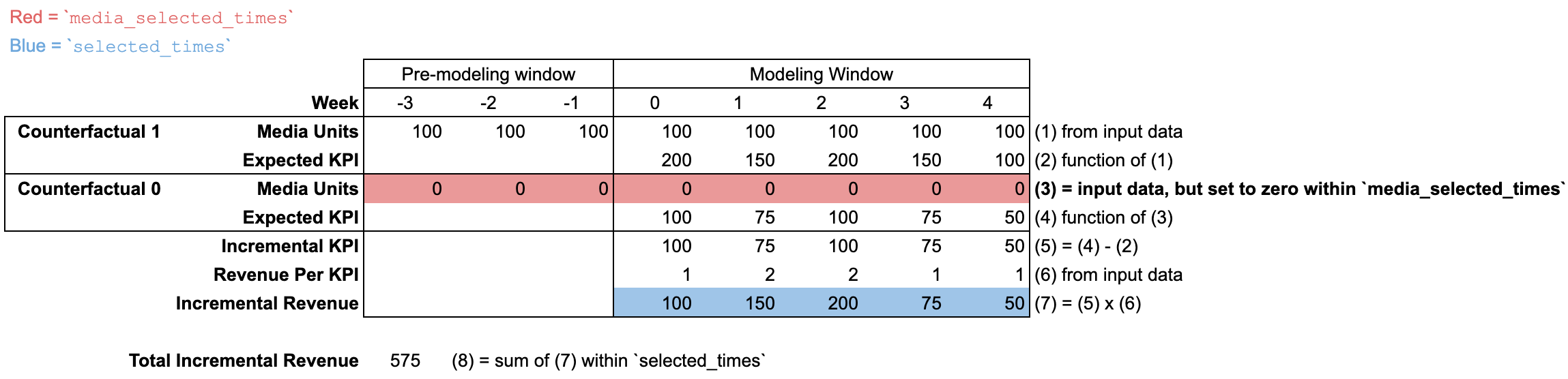
Incremental outcome

For each media channel, the incremental_outcome method compares the expected outcome under two counterfactual scenarios. In one scenario, the media units are set to the historical values. In the other scenario, the media units are set to zero for some or all time periods.

The media_selected_times argument determines the time periods over which the media units are set to zero.

The selected_times argument determines the time range over which the incremental outcome is measured.

Using input_data

The default incremental outcome definition sets media_selected_times to be all time periods, including both the "modeling window" and "pre-modeling window". (The input_data media units can optionally include a "pre-modeling window", which allows the model to properly take into account the lagged effect of these units.)

The default selected_times is all time periods in the "modeling window", which means that the incremental outcome is aggregated over all time periods in the "modeling window".

The input_data may contain media units during a "pre-modeling window" to account for lagged effects. The "pre-modeling window" does not contain any data besides media units, which is why cells are blank in the illustration.

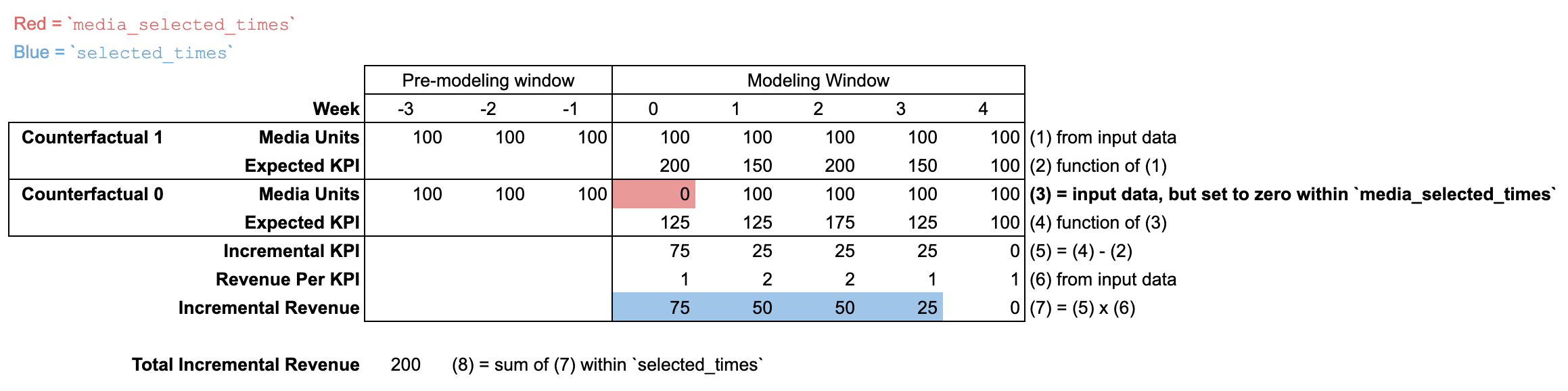
Using input_data with modified selected_times and media_selected_times

In order to understand the use of new_data in incremental_outcome and other methods, it is important to understand the selected_times and media_selected_times arguments.

In this example, media_selected_times is set to a single time period (week 0). Meanwhile, selected_times is set to be weeks 0 through 3. This example illustrates a scenario where max_lag is set to 3 in the ModelSpec, so the incremental outcome must be zero for weeks 4 and beyond. As a result, this combination of media_selected_times and selected_times captures the full long term impact of the week 0 media units.

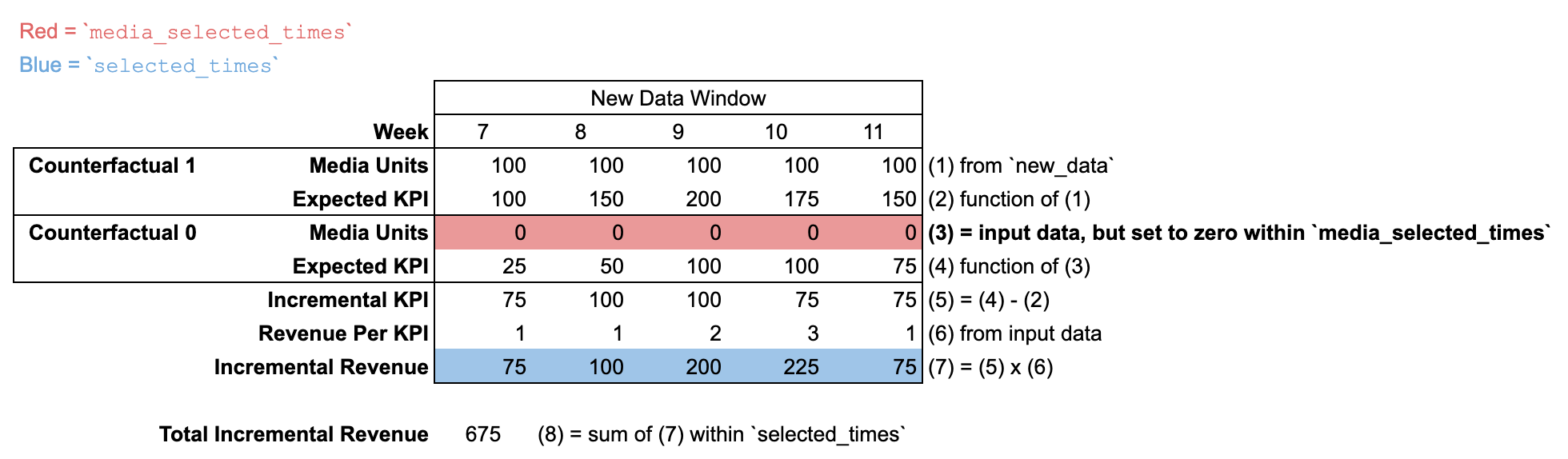
Using new_data with a new time window

When new_data is passed with a different number of time periods than the input_data, then there is no "pre-modeling window". It is assumed that media units are zero for all time periods prior to the new_data time window.

The default incremental outcome definition sets both media_selected_times and selected_times to be all time periods in the new_data time window.

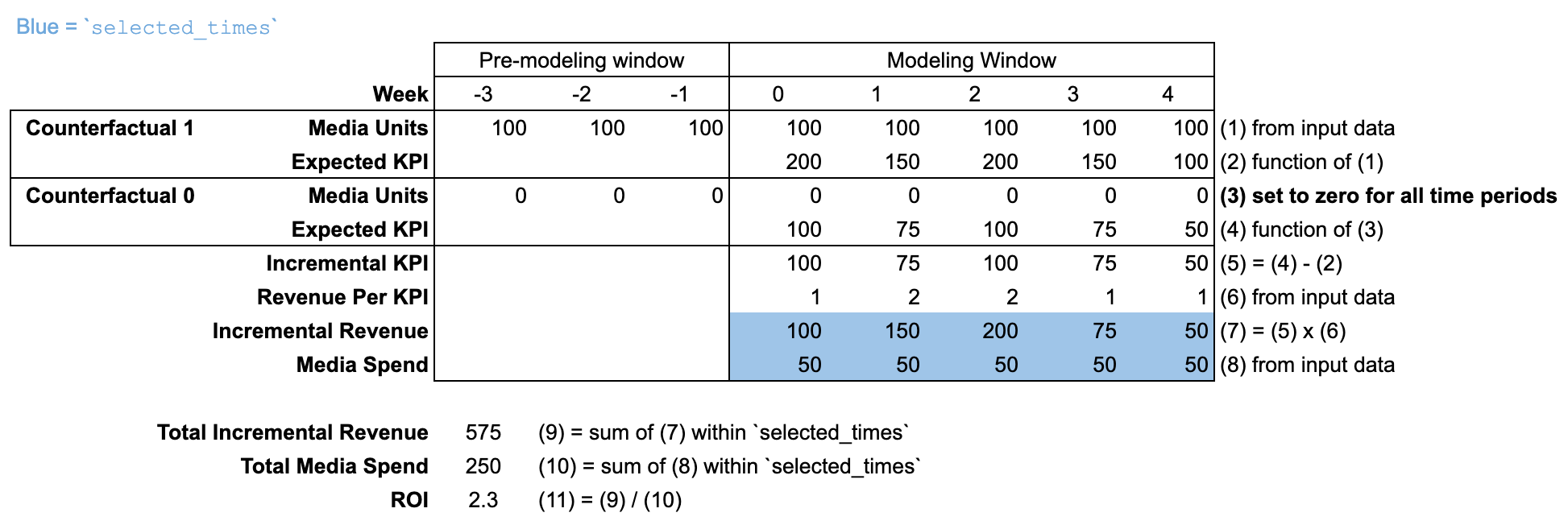
ROI

For each media channel, the roi method divides the incremental outcome generated during selected_times by the spend during selected_times. The roi method does not have a media_selected_times argument. The incremental outcome compares the counterfactual where media units are set to historical values against the counterfactual where media units are set to zero for all time periods.

Using input_data

By default, selected_times is set to the entire "modeling window". The counterfactual sets media units to zero for all time periods in both the "modeling window" and "pre-modeling window".

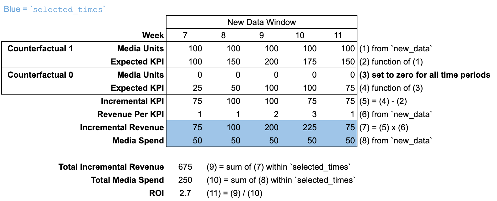
Using new_data with a new time window

When new_data is passed with a different number of time periods than the input_data, then there is no "pre-modeling window". It is assumed that media units are zero for all time periods prior to the new_data time window.

Response curves and budget optimization

The response_curves method is similar to roi in that the incremental outcome and spend are both aggregated over selected_times, which is set to the entire "modeling window" by default. Each point on the response curve x-axis is some percentage of the historical spend within the selected_times range. This method calculates the corresponding incremental outcome (y-axis) by scaling the historical media units by the same factor. The scaling factor is applied to the media units of both the "modeling window" and "pre-modeling window".

Budget optimization is based on response curves, so the same illustration applies to both response curves and budget optimization. Note that BudgetOptimizer.optimize has deprecated the selected_times argument and now uses start_date and end_date arguments instead.

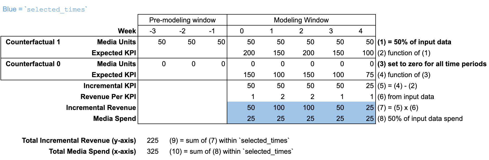
Using input_data

By default, selected_times is set to the entire "modeling window". The counterfactual sets media units are scaled for all time periods in both the "modeling window" and "pre-modeling window".

In this illustration, the response curve is calculated at 50% of the input_data budget.

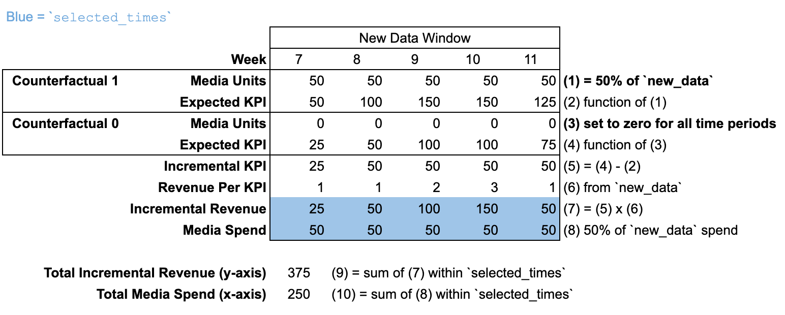
Using new_data with a new time window

When new_data is passed with a different number of time periods than the input_data, then there is no "pre-modeling window". It is assumed that media units are zero for all time periods prior to the new_data time window.

In this illustration, the response curve is calculated at 50% of the new_data budget.

Budget optimization code examples

The following examples illustrate the power of new_data for budget optimization and future scenario planning. For illustrative purposes, each example focuses on one key attribute of the input data that can be modified using new_data. However, all of these assumptions (and more) can be combined into one optimization scenario.

Imagine you want to optimize your budget for a future quarter that is expected to have a similar flighting pattern, cost per media unit, and revenue per KPI to the last quarter of input data. You can use the last quarter of input data to represent the future scenario and tweak the aspects that are expected to change. This is illustrated in the each of the examples.

In more complicated future scenarios, it might be better to entirely replace the input data with new data. This can either be done by constructing the arrays in Python, or by loading the data from a csv file.

In these examples, there are three media channels. The KPI is sales units, and revenue_per_kpi is provided. For the sake of illustration, each example runs an optimization scenario that is based on the fourth quarter of 2024. A key element of the scenario is modified in each example, and the new_data argument is used to incorporate the change.

The code in each example assumes that a Meridian model has been initialized as mmm, the sample_posterior method has been called, and a BudgetOptimizer has been initialized as opt.

mmm = model.Meridian(...)
mmm.sample_posterior(...)
opt = optimizer.BudgetOptimizer(mmm)

Example 1 - new cost per media unit for a single channel

Suppose the cost per media unit on the first channel is expected to double in the near future, so you want to double the assumed cost per media unit of this channel in the optimization. You can do this by creating a spend array that matches the input data, except the spend is doubled for the first channel. The array is passed to the DataTensors constructor, which in turn is passed to the new_data argument of the optimization.

Modifying the media_spend also affects the default total budget for fixed budget optimization, as well as the default spend constraints. These defaults can be overridden using the budget and pct_of_spend optimization arguments. It's important to be aware of these arguments and customize them as needed.

# Create `new_data` from `input_data`, but double the spend for channel 0.
new_spend = mmm.input_data.media_spend
new_spend[:, :, 0] *= 2
new_data = analyzer.DataTensors(media_spend=new_spend)
# Run fixed budget optimization on the last quarter of 2024, using customized
# total budget and constraints.
opt_results = opt.optimize(
    new_data=new_data,
    budget=100,
    pct_of_spend=[0.3, 0.3, 0.4],
    start_date="2024-10-07",
    end_date="2024-12-30",
)

Example 2 - new cost per media for all channels

Suppose the cost per media unit is expected to change in the near future for all channels, so you want to change the assumed cost per media unit of all channels in the optimization. For each channel, the anticipated cost is a known constant and constant across geos and time periods. The create_optimization_tensors helper method, which creates a DataTensors object, is convenient for this task because the cost per media unit (cpmu) is a direct input.

The create_optimization_tensors method requires all optimization arguments to be passed. Either media or media_spend can be passed (with geo and time dimension) to specify the flighting pattern. The time dimension of all arguments to create_optimization_tensors must match (media cannot include additional time periods for lagged effects).

# Create `new_data` using the helper method. The cost per media unit (cpmu) is
# set to a constant value for each channel.
new_cpmu = np.array([0.1, 0.2, 0.5])
media_excl_lag = mmm.input_data.media[:, -mmm.n_times:, :]
new_data = opt.create_optimization_tensors(
    time=mmm.input_data.time,
    cpmu=new_cpmu,
    media=media_excl_lag,
    revenue_per_kpi=mmm.input_data.revenue_per_kpi,
)
# Run fixed budget optimization on the last quarter of 2024, using customized
# total budget and constraints.
opt_results = opt.optimize(
    new_data=new_data,
    budget=100,
    pct_of_spend=[0.3, 0.3, 0.4],
    start_date="2024-10-07",
    end_date="2024-12-30",
)

The same task could be accomplished by creating the DataTensors object directly. To do this, the spend is calculated by scaling the media units of each channel by the cost per media unit for that channel.

# Create `new_data` without the helper method.
# In this example, `mmm.n_media_times > mmm.n_times` because the `media` data
# contains additional lag history. These time periods are discarded to create
# the new spend data.
media_excl_lag = mmm.input_data.media[:, -mmm.n_times:, :]
new_spend = media_excl_lag * np.array([0.1, 0.2, 0.5])
new_data = analyzer.DataTensors(media_spend=new_spend)
# Run fixed budget optimization on the last quarter of 2024, using customized
# total budget and constraints.
opt_results = opt.optimize(
    new_data=new_data,
    budget=100,
    pct_of_spend=[0.3, 0.3, 0.4],
    start_date="2024-10-07",
    end_date="2024-12-30",
)

Example 3 - new revenue per KPI

Suppose the revenue per KPI (e.g. unit price or lifetime value) is expected to change in the near future. The new revenue per KPI assumption can be incorporated into the optimization. To be clear, this will change assumed revenue generated per incremental KPI unit, but it won't change the model fit on the KPI itself.

# Create `new_data` from `input_data`, but double the revenue per kpi.
new_data = analyzer.DataTensors(
    revenue_per_kpi=mmm.input_data.revenue_per_kpi * 2
)
# Run fixed budget optimization on the last quarter of 2024, using customized
# total budget and constraints.
opt_results = opt.optimize(
    new_data=new_data,
    budget=100,
    pct_of_spend=[0.3, 0.3, 0.4],
    start_date="2024-10-07",
    end_date="2024-12-30",
)

Example 4 - new flighting pattern

You may be considering a different future flighting pattern (relative allocation of media units across geos or time periods). One common reason to do this is if you plan to shift budget from one geo to another. Another common reason is to account for a new media channel introduced during the input data window. When a new channel is introduced, the historical flighting pattern has zero media units prior to the time period when the channel was introduced. If you plan to execute the new channel continuously in the future, then the zeros in the flighting pattern should be replaced by other values to better reflect the future planned flighting pattern.

In this example, imagine that the first media channel was introduced during the fourth quarter of 2024. Perhaps it had zero spend initially and ramped up throughout the quarter. However, in the future you expect to set a constant media units per capita across geos and time periods. The media argument of DataTensors is used to specify the flighting pattern. When specifying this argument for a geo model, it's often best to consider the intended flighting pattern in terms of media units per capita.

The exact number of media units per capita (100 in this example) does not affect the flighting pattern. The flighting pattern is the relative allocation of media units across geos and time periods, so the same flighting pattern could be achieved by assigning 10 units per capita, for example. However, the media units also affect the cost per media unit assumption, which is derived from the ratio of spend per media unit within each geo and time period. In this example, the new spend data is passed to achieve a cost per media unit of 0.1 for all geos and time periods.

Modifying the media_spend also affects the default total budget for fixed budget optimization, as well as the default spend constraints. These defaults can be overridden using the budget and pct_of_spend optimization arguments. It's important to be aware of these arguments and customize them as needed.

# Create new media units data from the input data, but set the media units per
# capita to 100 for channel 0 for all geos and time periods.
new_media = mmm.input_data.media.values
new_media[:, :, 0] = 100 * mmm.input_data.population.values[:, None]
# Set a cost per media unit of 0.1 for channel 0 for all geos and time periods.
new_media_spend = mmm.input_data.media_spend.values
new_media_spend[:, :, 0] = 0.1 * new_media[:, -mmm.n_times:, 0]
new_data = analyzer.DataTensors(
    media=new_media,
    media_spend=new_spend,
)
# Run fixed budget optimization on the last quarter of 2024, using customized
# total budget and constraints.
opt_results = opt.optimize(
    new_data=new_data,
    budget=100,
    pct_of_spend=[0.3, 0.3, 0.4],
    start_date="2024-10-07",
    end_date="2024-12-30",
)

Why Meridian doesn't forecast outcome

Meridian does not need to forecast the expected outcome into the future in order for its causal inference to be useful for future planning. In fact, Meridian has methods to help with future planning including the Optimizer class and many methods including roi, marginal_roi, and incremental_outcome. The new_data argument in these methods allows one to use Meridian's causal inference to estimate quantities for any hypothetical media execution or flighting pattern, including future execution.

Meridian's goal is causal inference. More precisely, the goal is to infer the incremental outcome that treatment variables have on the outcome. Using terms from the Glossary, we simplify the incremental outcome definition as

\[ \text{Incremental Outcome} = \text{Expected Outcome} - \text{Counterfactual} \]

where the meaning of counterfactual depends on the treatment type. (See the Glossary for more information, and see Incremental outcome definition for a more precise definition.)

Control variables have an influence on expected outcome, but not on incremental outcome (other than the effect controls have on debiasing media effects). This is because the Meridian model specifies that control variables have an additive effect on both "Expected Outcome" and "Counterfactual", which cancels in the difference. Forecasting expected outcome would require us to forecast the control data. This can be quite difficult as many controls are very noisy, unpredictable, and completely outside the control of an advertiser. Forecasting the control data would be orthogonal to the causal inference goals of Meridian because we can infer incremental outcome, and even optimize it, without necessarily forecasting the expected outcome.

Similarly, the temporal effects, parameterized by knots, are additive. As a result, "Expected Outcome" and "Counterfactual" depend on the knot values, but "Incremental Outcome" does not. Meridian's knot-based approach for modeling temporal patterns is not designed for forecasting. Instead, it's designed to offer a much more flexible model for temporal patterns which makes it a good fit for the causal inference problem.