In Required assumptions, it was stated that conditional exchangeability assumption holds if you assume a causal graph that meets the backdoor criterion.
A causal graph shows the relationship between variables. Variables are grouped into collections (nodes), and an arrow between nodes indicates that a causal effect might exist in the direction of an arrow. An arrow does not necessarily indicate that a causal relationship exists between every pair of variables, but it does indicate that a causal relationship cannot exist in the reverse direction for any pair of variables.
The backdoor criterion (Pearl, J., 2009) states that given a causal diagram, a set of variables \(Z\) satisfies the backdoor criterion relative to a treatment variable \(X\) and the response variable \(Y\) if both of the following are true:
- No node in \(Z\) is a descendant of \(X\), and
- \(Z\) blocks every path between \(X\) and \(Y\) that contains an arrow into \(X\)
Marketing mix modeling (MMM) is used to estimate the causal effect of paid media, organic media, and non-media variables on a KPI (such as sales). So paid media, organic media, and non-media are the treatment variables (\(X\)) and the KPI is the response variable (\(Y\)). To estimate this causal effect from an MMM regression, the MMM must condition on a carefully selected set of control variables that meets the backdoor criterion. To paraphrase the backdoor criterion conditions:
- You must not control for any mediators. Mediators are variables that lie in the causal pathway between \(X\) and \(Y\).
- You must control for all confounders. Confounders are variables that have a causal effect on both \(X\) and \(Y\).
The MMM treatment variable is a collection of any combination of paid media, organic media, and non-media treatment variables indexed over both geo and time. It is is unwieldy to represent the entire treatment in a graph, so consider a simplified graph that represents only two time periods within a single geo. Geos are assumed to be independent, so the same graph can be used to represent any geo, and there are no arrows or relationships between geos. Two time periods are enough to describe the pattern of lagged treatment effects, which you can assume is repeated indefinitely into the future (or up to some maximum lag duration).
Meridian's causal graph
In the following diagram, \(T\) denotes paid media, organic media, and non-media treatment variables, \(C\) denotes controls, and \(K\) denotes the KPI. The number following each variable denotes the time period. Within each time period, assume that treatment affects sales, and that controls affect both treatment and sales. In the following diagram, \(T\) from a previous time period affects sales in the current time period ("lagged effect"). The Meridian regression model applies adstock to paid and organic media, but not to non-media treatments. This effectively assumes that non-media treatments don't have lagged effects. Including non-media treatments in node \(T\) is still valid because an arrow indicates that a causal effect may exist between any pair of variables in connected nodes. Including non-media treatments in node \(T\) makes the DAG presentation cleaner, and the DAG is still valid for determining which variables satisfy the backdoor criterion.
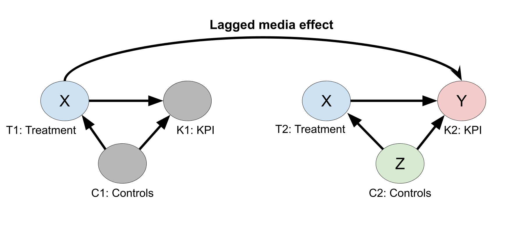
Consider the task of estimating the causal effect of treatment (\(T1\) and \(T2\)) on the KPI for time period 2 (\(K2\)). From the graph, you can see that the time 2 controls (\(C2\)) satisfies the backdoor criterion.
The main conclusions are that for each time period, the MMM regression should condition on:
- Paid and organic media from the current time period and all preceding time periods, up to an assumed maximum lag duration.
- Non-media treatment variables of the current time period only.
- Control variables of the current time period only.
A few noteworthy details to consider are:
- An arrow from \(C1\) to \(C2\) has no implication on which variables to include in the regression.
- An arrow from \(C1\) to \(K2\) requires the regression to include lagged control variables. In practice, it is best to avoid this if at all possible, as it could significantly increase the number of regression parameters.
- An arrow from \(T1\) to \(C2\) is problematic. In this case, \(C2\) is both a mediator and a confounder. A single MMM regression model cannot be used to recover the causal joint treatment effect.
- Adding the path \(T2 \leftarrow K1 \rightarrow K2\) is problematic for the same reason. In this case, \(K1\) acts as both a mediator and confounder.
Meridian can also support a causal graph with lagged controls, as discussed in When lagged controls are needed.
Meridian's full-funnel causal graph
To resolve the mediator-confounder dilemma, Meridian supports a full-funnel causal graph using a two-stage approach (see Full-Funnel MMM).
Single time period
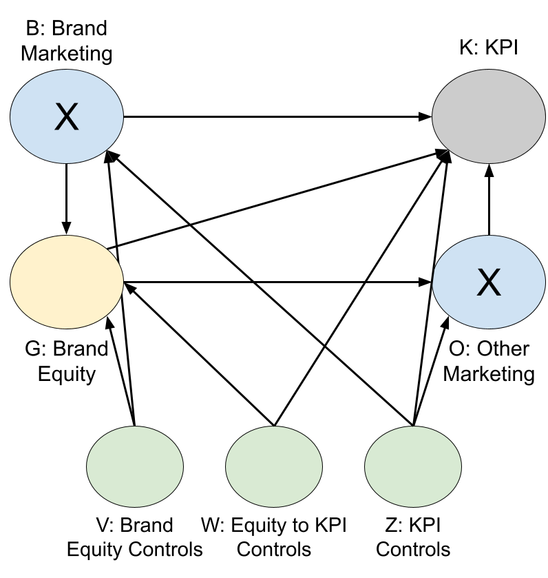
In the diagram, we see the full-funnel causal graph within one time point.
Treatment variables are split into two nodes:
- \(B\) denotes Brand marketing, which is marketing expected to influence the brand equity variable \(G\)
- \(O\) denotes other marketing, which is marketing that may be influenced by the brand equity variable \(G\).
Practically, it is helpful to identify which marketing variables are considered Brand marketing by asking: "Does this marketing variable have a causal effect on the brand equity variable?" If the answer is yes, it should be included in \(B\). If the answer is no, it should be included in \(O\). Recall that an arrow in a DAG represents a potential causal relationship. It does not require that the causal relationship truly exists. Therefore, each marketing variable in the \(O\) node does not necessarily need to be causally affected by the brand equity variable. For this reason, it is helpful to first determine the variables that should be classified as Brand marketing and then classify the remaining variables as Other marketing.
To give a concrete example, imagine we have branded GQV (bGQV) as a brand equity variable, categorizing it in the \(G\) node. A video ad channel is expected to drive brand equity and increase bGQV. We would consider the video ad channel a Brand marketing variable, categorizing it in the \(B\) node. On the other hand, a lower-funnel, performance-driven marketing channel is likely to be driven by brand equity. Thus, we would consider this Other marketing, categorizing it in the \(O\) node. For more on this example, see the Meridian Full-Funnel walkthrough.
Control variables are also split into three nodes:
- \(V\) denotes variables that confound with both Brand marketing and the brand equity variable \(G\).
- \(Z\) denotes variables that confound with marketing (whether Brand or Other) and the KPI \(K\).
- \(W\) denotes variables that confound with brand equity and the KPI \(K\).
Each of \(V\), \(Z\), and \(W\) are confounders for a causal effect we estimate in the full-funnel model: \(V\) are confounders for the causal effect Brand marketing has on the brand equity variable, \(Z\) are confounders for the causal effect marketing has on the KPI, and \(W\) are confounders for the causal effect brand equity has on the KPI. Just as in a single-stage MMM, it is important to consider confounders for all estimated causal effects.
Multiple time periods with lagged effects
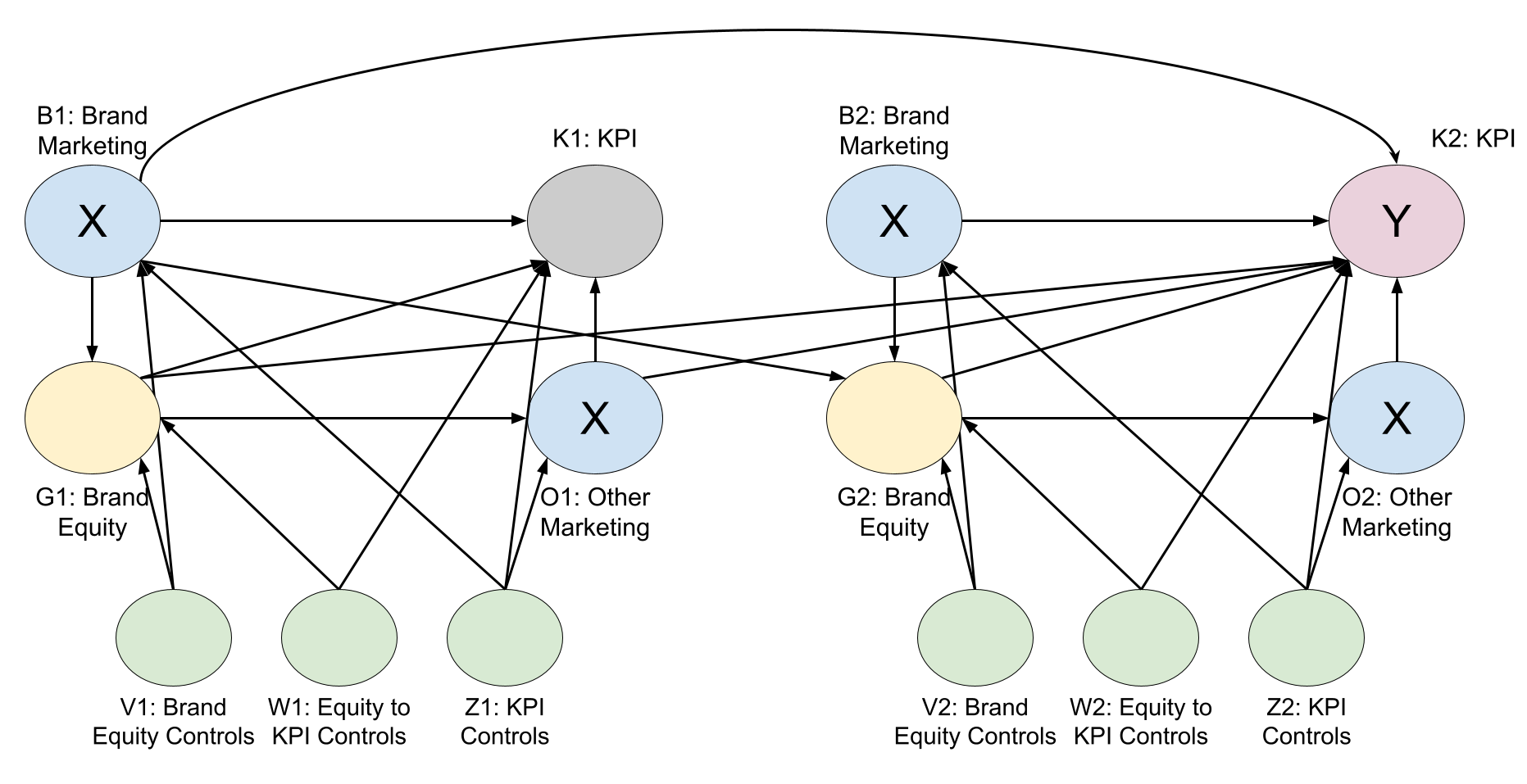
In the following diagram, multiple time periods are incorporated into the graph, with the number following each node's name denoting the time period. This adds a diagram for the following lagged effects assumed in Meridian's full-funnel causal graph:
- Brand marketing \(B\) on the KPI \(K\)
- Other marketing \(O\) on the KPI \(K\)
- Brand equity \(G\) on the KPI \(K\)
- Brand marketing \(B\) on Brand equity \(G\)