Analyze Site Performance with Places Insights and BigQuery ML

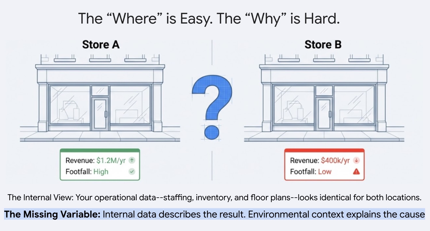
Why does one site thrive while another underperforms despite consistent staffing, inventory and operational practices? Businesses with multiple locations often struggle to explain this performance variance across their portfolio. The answer usually lies hidden in the external environment. By leveraging points of interest (POI) data, we can move beyond anecdotal explanations and quantify exactly how local competitive density and neighborhood characteristics dictate a site's success.

This guide demonstrates how to quantify the impact of local surroundings on site success using Places Insights and BigQuery ML. You will combine your proprietary site performance data with external geospatial signals to diagnose performance drivers.

We will use a dataset of sites in London to build a Linear Regression model. This workflow utilizes H3 Spatial Indexing, this system divides the city into uniform hexagonal cells. By aggregating environmental data into these cells, you can train a model to predict the performance potential of any neighborhood in the city, not just your existing sites.

You will learn to:

1. Engineer Features: Aggregate counts of Points of Interest (POIs) like gyms, schools, and transit stations within a 500-meter radius of your sites.
2. Train a Model: Use BigQuery ML to build a regression model that correlates these environmental features with your internal performance metrics.
3. Score the City: Apply the trained model to the entire H3 grid of London to identify high-potential hotspots for future expansion.

If you are new to BigQuery ML, see Introduction to BigQuery ML to learn about core concepts and supported model types.

To explore this workflow in an interactive environment, run the following notebook. It demonstrates how to build a predictive model with BigQuery ML and visualize city-wide opportunities using H3 spatial indexing.

Run in Google Colab

View source on GitHub

Prerequisites

Before you begin, ensure you have the following:

• Google Cloud Project:

  • A Google Cloud project with billing enabled.

• Data Access:

  • Places Insights subscription in BigQuery.
  • Your own table of site locations with a performance metric (e.g., revenue). An example dataset is in the tutorial resources.

• Google Maps Platform:

  • An API Key.
  • The following APIs enabled for your key:
    • Maps JavaScript API
    • Maps Tiles API

• Python Environment & Libraries:

  • A Python environment such as Colab Enterprise in the Google Cloud Console.
  • The following libraries installed:

    Library	Description
    pandas-gbq	Interacting with BigQuery.
    geopandas	Handling geospatial data operations.
    folium	Creating interactive maps.
    shapely	Geometric manipulations.

• IAM Permissions:

  • Ensure your user or service account has the following IAM roles:

    Role	ID
    BigQuery Data Editor	roles/bigquery.dataEditor
    BigQuery User	roles/bigquery.user

• Cost Awareness:

  • This tutorial uses billable Google Cloud components. Be aware of potential costs related to:
    • BigQuery ML: Charged for compute slots used. See BigQuery ML pricing.
    • Places Insights: Charged based on query usage.

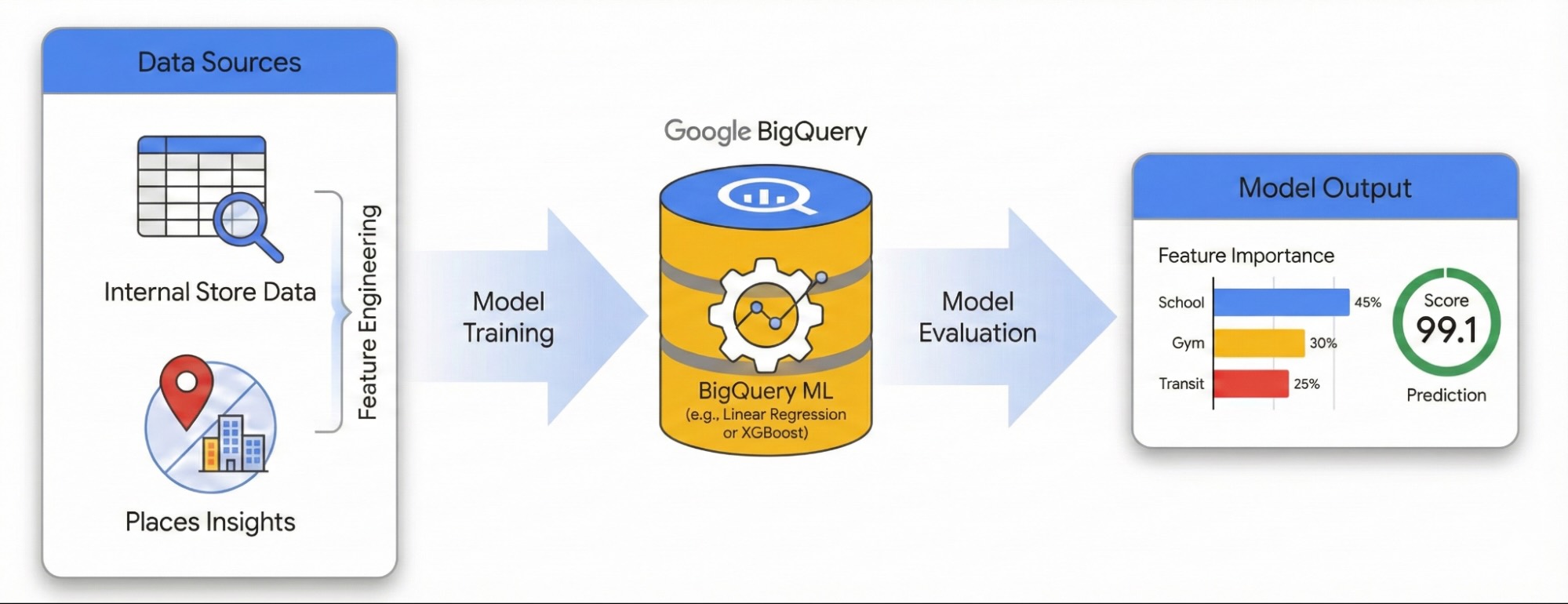
Feature Engineering with Places Insights

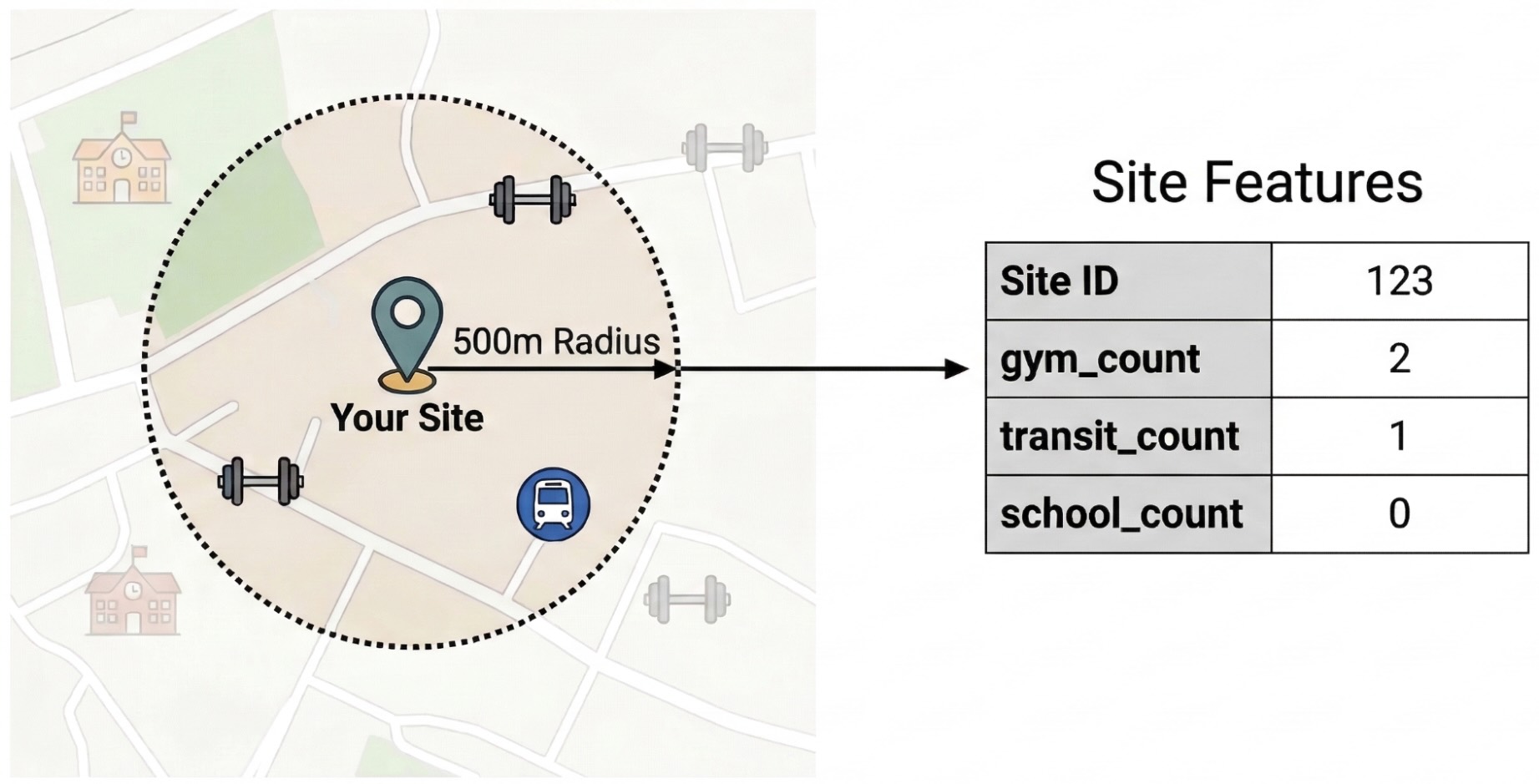
To isolate the external factors driving site performance, you must transform raw POI data into quantifiable features. You will calculate the density of specific amenities or types of places such as gyms, schools, and transit stations within a 500-meter radius of each site. The amenities you select will be dependent on what you believe may be most relevant for your business.

We use Python and the pandas-gbq library for this step. This approach lets you execute the SELECT WITH AGGREGATION_THRESHOLD query, which is required to access the Places Insights dataset, and save the results to a new table in your project. See Query the dataset directly for more information on working with Places Insights data.

Run the Feature Engineering Query

Run the following Python script in your environment (e.g., Colab Enterprise). This script connects your internal site data with the Places Insights dataset.

from google.cloud import bigquery
import pandas_gbq

# Configuration
project_id = 'your_project_id'
dataset_id = 'your_dataset_id'
features_table_id = f'{dataset_id}.site_features'

client = bigquery.Client(project=project_id)

# Define the Feature Engineering Query
# We count specific amenities within 500m of each site in London.
sql = f"""
SELECT WITH AGGREGATION_THRESHOLD
    internal.store_id,
    internal.store_performance,

    -- Feature Engineering: count nearby POIs by type
    COUNTIF('gym' IN UNNEST(places.types)) AS gym_count,
    COUNTIF('restaurant' IN UNNEST(places.types)) AS restaurant_count,
    COUNTIF('school' IN UNNEST(places.types)) AS school_count,
    COUNTIF('transit_station' IN UNNEST(places.types)) AS transit_count,
    COUNTIF('clothing_store' IN UNNEST(places.types)) AS clothing_store_count

FROM
    `{dataset_id}.site_performance` AS internal
JOIN
    `places_insights___gb.places` AS places
    ON ST_DWITHIN(internal.location, places.point, 500)
WHERE
    places.business_status = 'OPERATIONAL'
GROUP BY
    internal.store_id, internal.store_performance
"""

print("1. Running Feature Engineering Query...")

# Execute the query and download results to a Pandas DataFrame
df_features = client.query(sql).to_dataframe()

print(f"2. Saving features to: {features_table_id}...")

# Upload the engineered features to a permanent BigQuery table
pandas_gbq.to_gbq(
    dataframe=df_features,
    destination_table=features_table_id,
    project_id=project_id,
    if_exists='replace'
)

print("   Success! Training data ready.")

Understand the Query

1. ST_DWITHIN: This geospatial function creates a 500-meter buffer around each site location and identifies all Places Insights points that fall within that radius.
2. COUNTIF: This function calculates the density of specific place types (e.g., 'gym', 'school') for each site. These counts become the input features (X) for the machine learning model.
3. pandas_gbq.to_gbq: This function persists the query results into a new table (site_features). This permanent table serves as the clean training dataset for the BigQuery ML model.

For more advanced real-world applications, consider calculating features at multiple distances (e.g., 250m, 500m, 1km) and exploring other Places Insights attributes like rating, price_level, or regular_opening_hours. See supported place types and the core schema reference for the full list of Places Insights attributes.

Train the Model with BigQuery ML

With the engineered features saved in your site_features table, you can now train a Linear Regression model.

This model learns the optimal weights (β) for each environmental feature (X) to predict your site's performance (Y).

Handle Outliers with Robust Scaling

Geospatial data often contains extreme outliers that can distort standard linear models. For example, a site in London's West End might have 200 restaurants within 500 meters, while a suburban site has only 2. If you use standard scaling (Mean/Standard Deviation), the outlier (200) skews the distribution and forces the model to prioritize fitting that extreme value.

To solve this, we use Robust Scaling (ML.ROBUST_SCALER) within the model definition. This technique scales features based on the Median and Interquartile Range (IQR), making the model resilient to outliers and ensuring it learns from the typical distribution of your sites.

Create the Model

Run the following SQL query in BigQuery to create and train the model.

We use the TRANSFORM clause to apply robust scaling to all input features. We also set optimize_strategy = 'NORMAL_EQUATION' because it is the most efficient training method for relatively small datasets, like a typical portfolio of store locations. Finally, we filter out high-performing outliers (store_performance < 75) to focus the model on predicting typical growth patterns.

CREATE OR REPLACE MODEL `your_project.your_dataset.site_performance_model`
TRANSFORM(
  store_performance,
  -- Feature Engineering inside the model artifact
  -- These stats are calculated on the TRAINING split only
  ML.ROBUST_SCALER(gym_count) OVER() AS scaled_gym_count,
  ML.ROBUST_SCALER(restaurant_count) OVER() AS scaled_restaurant_count,
  ML.ROBUST_SCALER(school_count) OVER() AS scaled_school_count,
  ML.ROBUST_SCALER(transit_count) OVER() AS scaled_transit_count,
  ML.ROBUST_SCALER(clothing_store_count) OVER() AS scaled_clothing_store_count
)
OPTIONS(
    model_type = 'LINEAR_REG',
    input_label_cols = ['store_performance'],

    -- OPTIMIZATION PARAMETERS
    optimize_strategy = 'NORMAL_EQUATION', -- Exact mathematical solution (fast for small data)
    data_split_method = 'AUTO_SPLIT',      -- Automatically reserves ~20% for evaluation

    -- DIAGNOSTICS
    enable_global_explain = TRUE -- Essential to see feature importance
)
AS
SELECT
    gym_count,
    restaurant_count,
    school_count,
    transit_count,
    clothing_store_count,
    store_performance
FROM
    `your_project.your_dataset.site_features`
WHERE
    store_performance < 75;

Evaluate Model Performance

Before you can trust the model's insights into what drives site performance, you must verify its predictions are accurate.

After training, use the ML.EVALUATE function to assess the model's predictions against a "holdout" set of data that was not used during training.

SELECT
  *
FROM
  ML.EVALUATE(MODEL `your_project.your_dataset.site_performance_model`);

Check the R2 Score (r2_score) and Mean Absolute Error (mean_absolute_error) to determine if your model is ready for production:

• An R2 score measures how much of the performance variance is actually explained by the external environmental factors (nearby POIs). An R2 score of 0.70 means 70% of a site's success is tied to the local environment. The closer to 1.0, the stronger the correlation between the environmental amenities and site performance.
• The MAE tells you the average error in points. For example, an MAE of 1.5 means the model's predictions are typically within +/- 1.5 points of the actual performance score.

Troubleshooting Low Scores

If your R2 score is low, consider the following improvements:

• Expand Feature Types: Add different Place Types to your query (e.g., tourist_attraction, subway_station).
• Adjust Catchment Radius: Change the ST_DWITHIN distance. A 500-meter radius might be too broad for a coffee shop but too small for a furniture store.
• Increase Data Size: Ensure you are training on enough store locations to find a statistically significant pattern.

Score the City with H3 Spatial Indexing

We use H3 Spatial Indexing to divide the city of London into a uniform grid of hexagonal cells (Resolution 8, approximately 0.7km²). By aggregating Places Insights data into these cells, we can apply our trained model to every neighborhood, identifying high-potential areas that match the environmental profile of your top-performing sites.

Run the Prospecting Query

To generate this grid, we use the PLACES_COUNT_PER_H3 function provided by the Places Insights dataset (Learn more about querying Places Insights using Places Count functions). This function calculates POI counts for H3 grid cells in a single operation.

Run the following SQL query to perform three steps in a single execution:

1. H3 Indexing & Counting: We call PLACES_COUNT_PER_H3 using a JSON configuration object to find all operational places within a 25km radius of central London. We query this separately for each amenity type (gyms, schools, etc.) and combine them using UNION ALL.
2. Pivoting (Feature Engineering): Because our machine learning model expects distinct feature columns (like gym_count and restaurant_count), we group the cells and use conditional aggregation (SUM(IF(...))) to pivot the data into the correct schema.
3. Prediction: We feed these pivoted grid features directly into the ML.PREDICT function to generate a performance score for every neighborhood.

WITH combined_counts AS (
    -- Gyms
    SELECT h3_cell_index, geography, count, 'gym' AS type
    FROM `places_insights___gb.PLACES_COUNT_PER_H3`(
        JSON_OBJECT(
            'geography', ST_BUFFER(ST_GEOGPOINT(-0.1278, 51.5074), 25000), -- 25km radius around London
            'h3_resolution', 8,
            'business_status', ['OPERATIONAL'],
            'types', ['gym']
        )
    )
    UNION ALL
    -- Restaurants
    SELECT h3_cell_index, geography, count, 'restaurant' AS type
    FROM `places_insights___gb.PLACES_COUNT_PER_H3`(
        JSON_OBJECT(
            'geography', ST_BUFFER(ST_GEOGPOINT(-0.1278, 51.5074), 25000),
            'h3_resolution', 8,
            'business_status', ['OPERATIONAL'],
            'types', ['restaurant']
        )
    )
    UNION ALL
    -- Schools
    SELECT h3_cell_index, geography, count, 'school' AS type
    FROM `places_insights___gb.PLACES_COUNT_PER_H3`(
        JSON_OBJECT(
            'geography', ST_BUFFER(ST_GEOGPOINT(-0.1278, 51.5074), 25000),
            'h3_resolution', 8,
            'business_status', ['OPERATIONAL'],
            'types', ['school']
        )
    )
    UNION ALL
    -- Transit Stations
    SELECT h3_cell_index, geography, count, 'transit_station' AS type
    FROM `places_insights___gb.PLACES_COUNT_PER_H3`(
        JSON_OBJECT(
            'geography', ST_BUFFER(ST_GEOGPOINT(-0.1278, 51.5074), 25000),
            'h3_resolution', 8,
            'business_status', ['OPERATIONAL'],
            'types', ['transit_station']
        )
    )
    UNION ALL
    -- Clothing Stores
    SELECT h3_cell_index, geography, count, 'clothing_store' AS type
    FROM `places_insights___gb.PLACES_COUNT_PER_H3`(
        JSON_OBJECT(
            'geography', ST_BUFFER(ST_GEOGPOINT(-0.1278, 51.5074), 25000),
            'h3_resolution', 8,
            'business_status', ['OPERATIONAL'],
            'types', ['clothing_store']
        )
    )
),
aggregated_features AS (
    -- Pivot the stacked rows back into standard feature columns for the ML Model
    SELECT
        h3_cell_index AS h3_index,
        ANY_VALUE(geography) AS h3_geography,
        SUM(IF(type = 'gym', count, 0)) AS gym_count,
        SUM(IF(type = 'restaurant', count, 0)) AS restaurant_count,
        SUM(IF(type = 'school', count, 0)) AS school_count,
        SUM(IF(type = 'transit_station', count, 0)) AS transit_count,
        SUM(IF(type = 'clothing_store', count, 0)) AS clothing_store_count
    FROM
        combined_counts
    GROUP BY
        h3_cell_index
)

-- Feed the pivoted features into the model
SELECT
    h3_index,
    predicted_store_performance,
    h3_geography,
    gym_count,
    restaurant_count
FROM
    ML.PREDICT(MODEL `your_project.your_dataset.site_performance_model`,
      (SELECT * FROM aggregated_features)
    )
ORDER BY
    predicted_store_performance DESC;

Interpret the Results

The query returns a table where each row represents a hexagonal area in London.

• h3_index: The unique identifier for the hexagonal cell.
• predicted_store_performance: The model's estimated score for a site located in this cell, based solely on the surrounding environment.
• h3_geography: The polygon geometry of the cell, which we will use for visualization in the next step.

High values indicate areas where the density of schools, gyms, and transit matches the patterns found around your most successful existing sites.

Visualize the Prospecting Map

To make the data actionable, visualize the results on a map. While the tabular output provides raw scores, a map reveals spatial clusters and corridors of high potential that are not obvious in a list.

In the accompanying notebook, we use the geopandas library to parse the H3 polygon geometry and folium to render an interactive map.

The result is a choropleth map where every hexagonal cell is colored according to its predicted score.

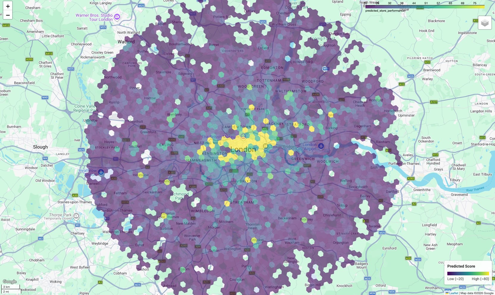
Interpret the Map:

• Hotspots (Yellow/Green): These areas have high predicted performance scores. They possess the optimal density of schools, gyms, and transit that correlates with your successful sites. These are prime candidates for new site selection.
• Coldspots (Purple): These areas lack the supporting environmental features found near your top performers.
• Interactive Inspection: In the notebook environment, you can hover over any cell to see the specific counts of amenities (e.g., "Gyms: 12") that contributed to that specific score.

Conclusion

You have successfully combined internal operational data with Places Insights to diagnose site performance. By analyzing the model weights, you identified the specific neighborhood characteristics that correlate with your existing metrics. Using H3 spatial indexing, you scaled this analysis from a few hundred sites to thousands of potential neighborhoods across London.

Next Actions

• Expand Feature Engineering: Add more specific Place Types to your query, to capture niche drivers of foot traffic.
• Explore Advanced Models: While Linear Regression provides clear explainability, experiment with BOOSTED_TREE_REGRESSOR in BigQuery ML combined with an appropriate cross-validation strategy to capture non-linear relationships.
• Operationalize the Map: Export the H3 grid results to a custom dashboard using the Maps JavaScript API to share these insights with your team.

Contributors

• Henrik Valve | DevX Engineer
• Gennadii Donchyts | Staff Customer Engineer