Page Summary
-
Visualize large location datasets on Google Maps with performant rendering using Google Cloud and Google Maps Platform.
-
Leverage BigQuery to query and process location data, exporting it to Google Cloud Storage for use with the Datasets API.
-
Create and style map visualizations with the Datasets API and Maps JavaScript API, enabling dynamic styling and interactivity.
-
Optimize data for performance by pruning properties, simplifying geometries, and using efficient data types.
-
This architecture supports various use cases, including visualizing open data, telecom coverage, and vehicle fleet movement.
This document provides a reference architecture and example for creating map data visualizations with location data in Google Cloud BigQuery and Google Maps Platform Datasets API, such as analyzing open municipal data, creating a telecommunication coverage map, or visualizing traces of mobile vehicle fleet movement.
Map data visualizations are a powerful tool to engage users and uncover spatial insights in location data. Location data is data that has point, line, or polygon features. For example, weather maps help consumers understand and plan trips and prepare for storms; business intelligence maps help users uncover insights from their data analysis, and telecommunications maps help users understand their providers' coverage and quality in a given service area.
However, it's difficult for app developers to make large map data visualizations that are performant and provide a great user experience. Large data must be loaded into memory client side, causing slow first map load times. The visual must be performant on all devices including lower-end mobile phones which have memory and GPU constraints. Finally developers need to choose a large data rendering library that is portable, reliable, and performant with large data.
Reference Architecture
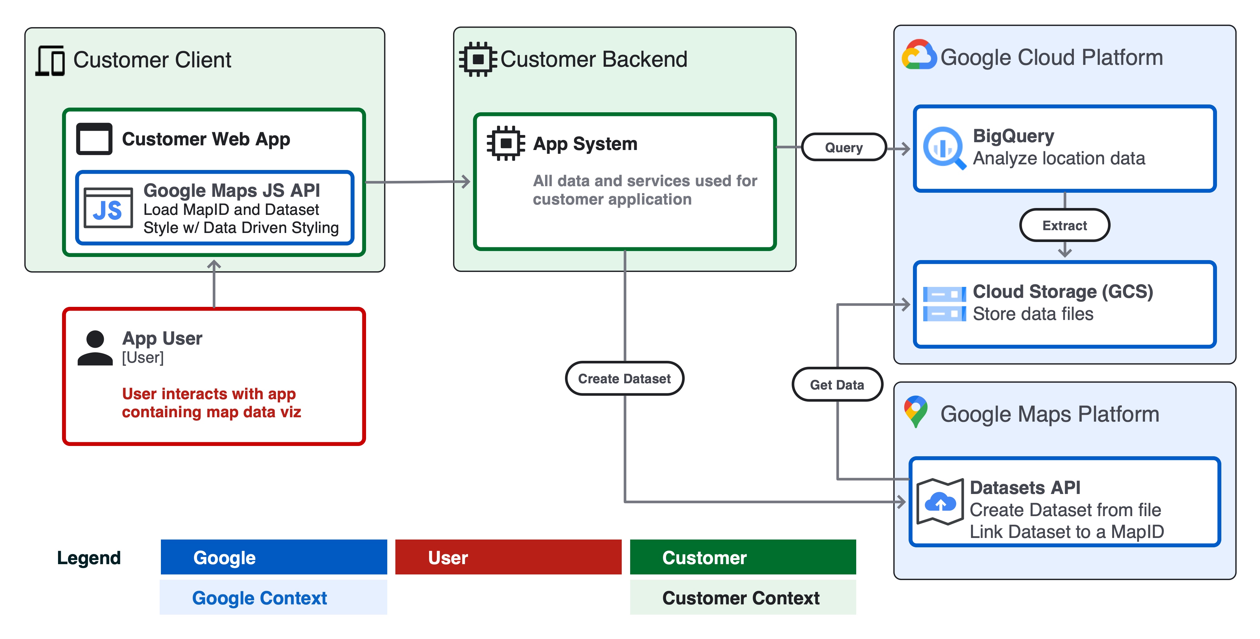
Developing apps with large data visualizations requires two main components.
- Customer backend - all backend app data & services such as processing and storage.
- Customer client - Your app user interface with a map visualization component.
Below is a system diagram of how these two components interact with the app user, Google Cloud, and Google Maps Platform to create a large data visualization app.

Design considerations
There are a number of design considerations to follow to create a performant data visualization using Google Cloud and Google Maps Platform.
- Source data size and update frequency.
- If the source data in geojson format is <5mb or updates very frequently e.g. a live weather radar forecast, consider serving data as a geojson object client side in your app and render with a deck.gl layer.
- If your data is more than 5mb in size and updates no faster than one time per hour, consider the Datasets API architecture in this document.
- Datasets support files up to 350 mb in size.
- If your data is larger than 350mb, consider pruning or simplifying geometry data in the source file before passing to Datasets (see Data Pruning below).
- Schema & format
- Ensure your data has a globally unique ID property for each feature. A unique ID allows you to select and style a specific feature or join data to a feature to visualize, for example styling a selected feature on the “click” user event.
- Format your data as CSV or GeoJSON according to the Datasets API spec with valid column names, data types, and types of GeoJSON objects.
- For easy creation of Datasets from BigQuery, create a column named
wktin your SQL CSV export. Datasets supports importing geometry from a CSV in Well-Known Text (WKT) format from a column namedwkt. - Check that your data is valid geometry and data types. For example, GeoJSON must be in the WGS84 coordinate system, geometry winding order, etc.
- Use a tool like geojson-validate to ensure all geometries in a source file are valid or ogr2ogr to transform a source file between formats or coordinate systems.
- Data pruning
- Minimize the number of properties of features. You can join additional properties to a feature at runtime on a unique identifier key (example).
- Use integer data types for property objects where possible to minimize tile storage space, keeping tiles performant to load over HTTPS in a client app.
- Simplify and/or aggregate very complex feature geometries; consider using BigQuery functions like ST_Simplify on complex polygon geometries to reduce source file size and improve map performance.
- Tiling
- Google Maps Datasets API creates map tiles from your source data file for use with a web or mobile Maps SDK.
- Map tiles are a zoom-based indexing system that provides more efficient ways of loading data into a visual app.
- Map tiles may drop dense or complex features at lower zoom levels. When a user zooms out to a state or country (e.g. z5-z12) may look different than when zoomed into a city or neighborhood (e.g. z13-z18).
Example - Railways in London
In this example, we'll apply the reference architecture to create a web application with Google Cloud and Google Maps that visualizes all railways in London from Open Street Map (OSM) data.
Prerequisites
- Access to BigQuery Sandbox and Cloud Console
- Ensure you have a Google Cloud project and billing account setup.
Step 1 - Query data in BigQuery
Navigate to BigQuery Public
Datasets. The dataset
'bigquery-public-data' and table geo_openstreetmap.planet_features contains
the entire globe's worth of Open Street Map
(OSM) data including all possible features. Discover all of the available
features to query in the OSM
Wiki including amenity,
road, and landuse.
Use Cloud Shell or the BigQuery Cloud Console to query the table using SQL. The code snip below uses the bq query command to query all the railways filtered to just London by using a bounding box and the ST_Intersects() function.
To perform this query from Cloud Shell, run the following code snip, updating the project ID, dataset, and table name for your environment.
bq query --use_legacy_sql=false \
--destination_table PROJECTID:DATASET.TABLENAME \
--replace \
'SELECT
osm_id,
feature_type,
(SELECT value
         FROM   unnest(all_tags)
         WHERE  KEY = "name") AS name,
(SELECT value
         FROM   unnest(all_tags)
         WHERE  KEY = "railway") AS railway,
geometry as wkt
FROM   bigquery-public-data.geo_openstreetmap.planet_features
WHERE ("railway") IN (SELECT key FROM unnest(all_tags))
    AND ST_Intersects(
    geometry,
ST_MakePolygon(ST_MakeLine(
      [ST_GeogPoint(-0.549370, 51.725346),
      ST_GeogPoint(-0.549370, 51.2529407),
      ST_GeogPoint(0.3110581, 51.25294),
      ST_GeogPoint(0.3110581, 51.725346),
      ST_GeogPoint(-0.549370, 51.725346)]
    ))
   )'
The query returns:
- a unique identifier for each feature
osm_id - the
feature_typee.g. points, lines, etc - The
nameof the feature e.g.Paddington Station - The
railwaytype e.g. main, tourism, military, etc - The
wktof the feature - point, line, or polygon geometry in WKT format. WKT is the standard data format BigQuery Geography columns return in a query.
Note - To visually validate your query results before creating a Dataset, you can quickly visualize your data in a dashboard from BigQuery using Looker Studio.
To export the table to a CSV file in a Google Cloud Storage bucket, use the bq extract command in Cloud Shell:
bq extract \
--destination_format "CSV" \
--field_delimiter "," \
--print_header=true \
PROJECTID:DATASET.TABLENAME \
gs://BUCKET/FILENAME.csv
Note: you can automate each step using Cloud Scheduler to update your data regularly.
Step 2 - Create a Dataset from your CSV file
Next create a Google Maps Platform dataset from the query output on Google Cloud Storage (GCS). Using the Datasets API, you can create a dataset and then upload data to your Dataset from a file hosted on GCS.
To get started, enable the Maps Datasets API on your Google Cloud project and review the API docs. There are Python and Node.js client libraries for calling the Datasets API from logic in your app backend. Additionally, there is a Datasets GUI for creating Datasets manually in Cloud Console.
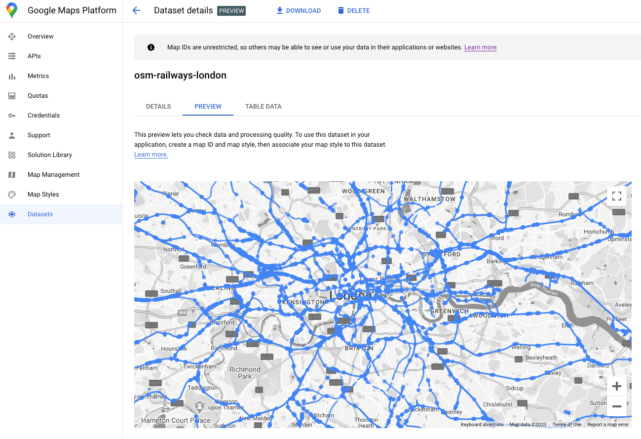
After your Dataset upload is complete, you can preview your dataset in the Datasets GUI.

Step 4 - Associate your Dataset with a map ID
Once your Dataset is created, you can create a map ID with an associated Map Style. In the Map Style editor, you can associate a mapId and style with the Dataset. This is also where you can apply Cloud Based Map Styling to customize the look and feel of your map.
Step 5 - Create your client app map visualization
Finally, you can add the dataset to a client-side data visualization app using the Maps JS API. Initialize your map object using the mapID associated with your dataset from the previous step. Then set the style and interactivity of your Dataset layer. Check out a complete guide to data driven styling with Datasets for more details.
You can customize the style, add event handlers for changing the style dynamically and more using the Maps JS API. See examples in the docs. Below we'll define a setStyle function to create the point and line feature style for this example based on the attribute "feature_type".
function setStyle(params) {
  const map.getDatasetFeatureLayer("your-dataset-id");
  const datasetFeature = params.feature;
  const type = datasetFeature.datasetAttributes["feature_type"];
if (type == "lines") {
           return {
             fillColor: "blue",
             strokeColor: "blue",
             fillOpacity: 0.5,
             strokeWeight: 1,
           }
         } else if (type == "points") {
           return {
             fillColor: "black",
             strokeColor: "black",
             strokeOpacity: 0.5,
             pointRadius: 2,
             fillOpacity: 0.5,
             strokeWeight: 1,
           }
     }
}
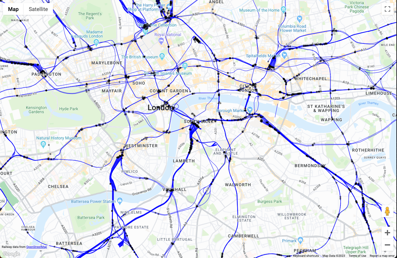
This code above when initialized in a single page web app yields the following map data visual:

From here, you can extend your map visualization in the setStyle() function by
adding logic to filter features, add styling based on user interaction, and
interacting with the rest of your application.
Conclusion
In this document, we discussed a reference architecture and example implementation of a large data visualization application using Google Cloud and Google Maps Platform. Using this reference architecture, you can create location data visualization apps from any data in Google Cloud BigQuery that are performant on any device using the Google Maps Datasets API.
Next Actions
Further reading:
- Google Maps Platform Datasets API documentation
- See your data in real time with Data Drive Styles
- Introduction to geospatial analytics in BigQuery
- Using GeoJSON in BigQuery for geospatial analytics
Contributors
Principal authors:
- Ryan Baumann, Google Maps Platform Solutions Engineering Manager
