运行模型诊断

构建模型后，您必须评估收敛性，根据需要调试模型，然后评估模型拟合度。

评估收敛性

您可以评估模型收敛性，以帮助确保模型的完整性。

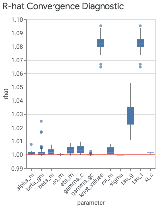
visualizer.ModelDiagnostics() 下的 plot_rhat_boxplot 命令会汇总并计算关于链收敛的 Gelman 和 Rubin（1992 年）潜在规模缩减，通常称为 R-hat。这种收敛诊断可以衡量链间（平均值）方差超出链同分布时预期方差的程度。

每个模型形参都有一个 R-hat 值。该箱线图汇总了各个索引中 R-hat 值的分布情况。例如，与 beta_gm x 轴标签对应的箱体汇总了地理位置索引 g 和渠道索引 m 中 R-hat 值的分布情况。

值接近 1.0 表示收敛。R-hat 值小于 1.2 表示近似收敛，对于许多问题来说，这是一个合理阈值（Brooks 和 Gelman，1998 年）。不收敛通常有以下两个原因：未能根据数据正确指定模型，这个问题可能存在于似然（模型规范）或先验中；或者是预选不足，也就是说 n_adapt + n_burnin 不够大。

如果您在实现收敛方面遇到问题，请参阅实现 MCMC 收敛。

生成 R-hat 箱线图

运行以下命令可生成 R-hat 箱线图：

model_diagnostics = visualizer.ModelDiagnostics(meridian)
model_diagnostics.plot_rhat_boxplot()

输出示例：

生成轨迹图和密度图

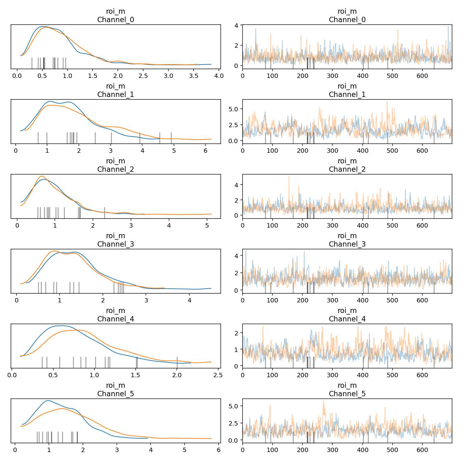
您可以为马尔可夫链蒙特卡洛 (MCMC) 样本生成轨迹图和密度图，帮助评估各链的收敛性和稳定性。轨迹图中的每个轨迹都表示 MCMC 算法在探索形参空间时生成的值序列。它展示了算法在连续迭代过程中如何处理不同的形参值。在轨迹图中，应尽量避免出现扁平区域，即链在很长时间内保持同一状态或在一个方向上有过多连续的步。

左侧的密度图直观呈现了通过 MCMC 算法获得的一个或多个形参的抽样值密度分布。在密度图中，您希望看到链已经收敛到平稳的密度分布。

以下示例展示了如何生成轨迹图和密度图：

parameters_to_plot=["roi_m"]
for params in parameters_to_plot:
  az.plot_trace(
      meridian.inference_data,
      var_names=params,
      compact=False,
      backend_kwargs={"constrained_layout": True},
  )

输出示例：

检查先验分布和后验分布

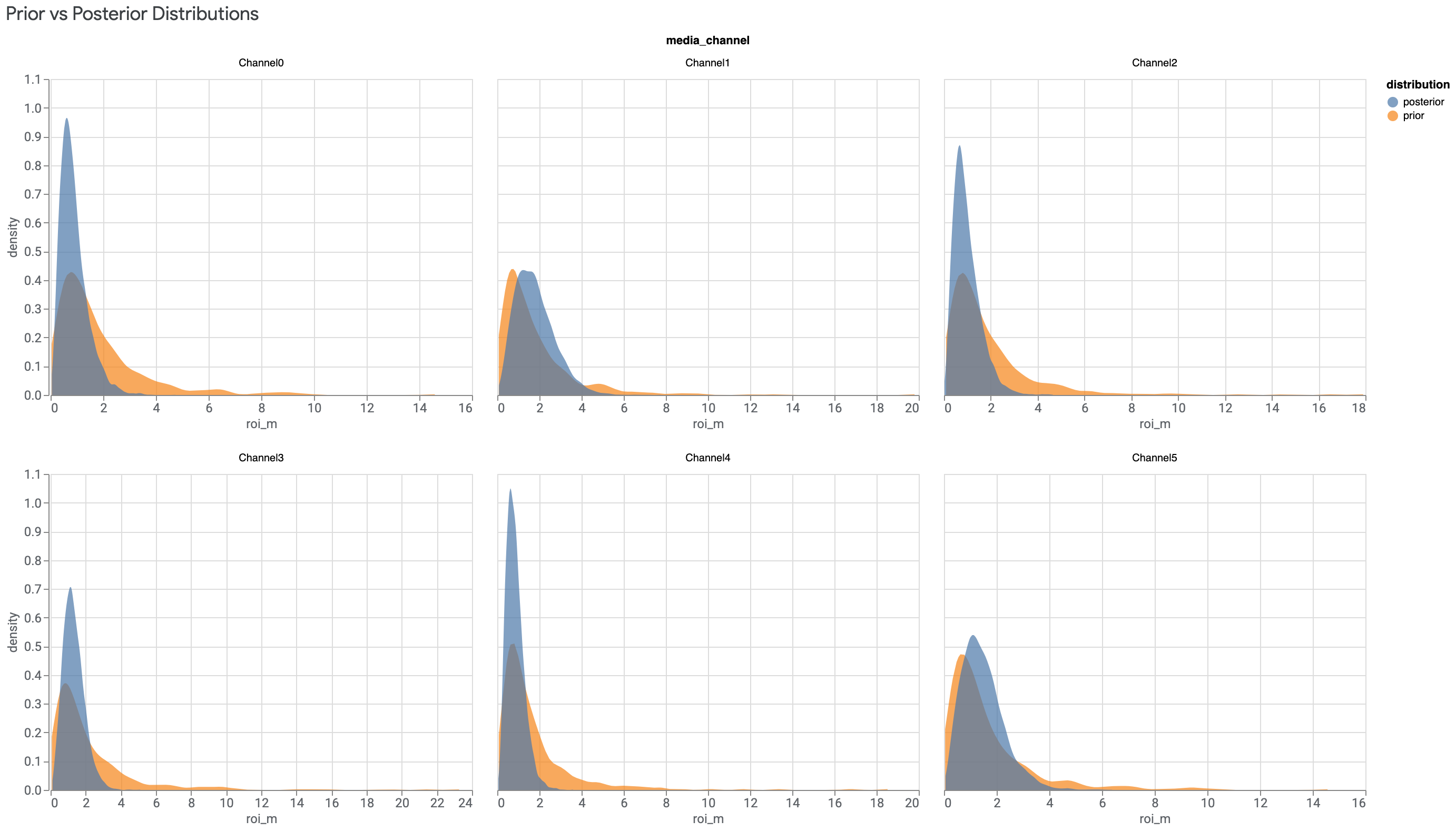
如果数据中的信息很少，先验和后验会相似。如需了解详情，请参阅后验与先验相同。

低支出渠道尤其容易出现与投资回报率先验相似的投资回报率后验。为了解决此问题，我们建议您在为 MMM 准备数据时舍弃支出非常低的渠道，或者将这些渠道与其他渠道合并。

运行以下命令可绘制每个媒体渠道的投资回报率后验分布与投资回报率先验分布对比图：

model_diagnostics = visualizer.ModelDiagnostics(meridian)
model_diagnostics.plot_prior_and_posterior_distribution()

输出示例：（点击图片可放大。）

默认情况下，plot_prior_and_posterior_distribution() 会生成投资回报率后验和先验。不过，您可以将特定模型形参传递给 plot_prior_and_posterior_distribution()，如以下示例所示：

model_diagnostics.plot_prior_and_posterior_distribution('beta_m')

评估模型拟合度

优化模型收敛性后，应评估模型拟合度。如需了解详情，请参阅“建模后”阶段中的评估模型拟合度。

使用营销组合建模分析 (MMM) 时，您必须依赖间接衡量方式来评估因果推理并寻找合理的结果。可以通过以下两种不错的方式实现这一点：

• 运行命令来生成 R 平方、平均绝对百分比误差 (MAPE) 和加权平均绝对百分比误差 (wMAPE) 指标
• 生成预期与实际收入或 KPI（具体取决于 kpi_type 以及是否有 revenue_per_kpi）对比图。

运行命令来生成 R 平方、MAPE 和 wMAPE 指标

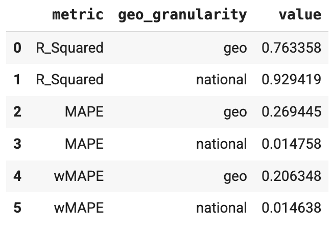
拟合优度指标可用作置信度检查指标，用于检查模型结构是否合适以及是否过度形参化。ModelDiagnostics 可计算 R-Squared、MAPE 和 wMAPE 拟合优度指标。如果在 Meridian 中设置了 holdout_id，还会对 Train 和 Test 子集计算 R-squared、MAPE 和 wMAPE。请注意，拟合优度指标用于衡量预测准确率，而预测准确率通常不是 MMM 的目标。不过，这些指标仍可作为实用的置信度检查指标。

运行以下命令可生成 R 平方、MAPE 和 wMAPE 指标：

model_diagnostics = visualizer.ModelDiagnostics(meridian)
model_diagnostics.predictive_accuracy_table()

输出示例：

生成预期与实际对比图

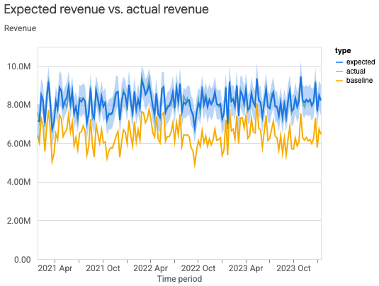
借助预期与实际对比图，可以间接评估模型拟合度。

国家：预期与实际对比图

您可以绘制国家级实际收入（或 KPI）与模型的预期收入（或 KPI）对比图，帮助评估模型拟合度。基准值是指在没有媒体执行的情况下，模型对收入（或 KPI）的反事实估计值。估计收入尽可能接近实际收入并不一定是 MMM 的目标，但它确实可以作为实用的置信度检查指标。

运行以下命令可根据国家级数据绘制实际收入（或 KPI）与预期收入（或 KPI）对比图：

model_fit = visualizer.ModelFit(meridian)
model_fit.plot_model_fit()

输出示例：

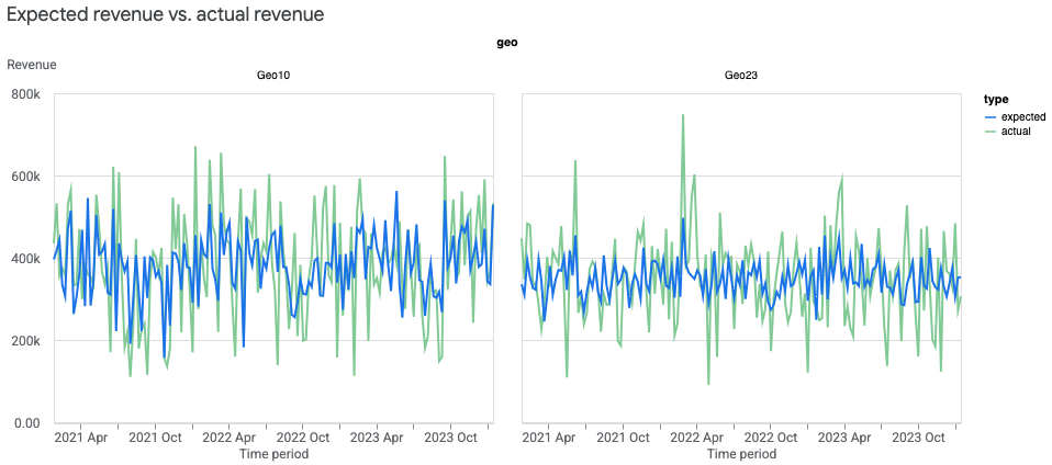
地理位置：预期与实际对比图

您可以创建地理位置级预期与实际对比图，帮助评估模型拟合度。由于地理位置可能很多，您可能希望只显示最大的地理位置。

运行以下命令可根据地理位置级数据绘制实际收入（或 KPI）与预期收入（或 KPI）对比图：

model_fit = visualizer.ModelFit(meridian)
model_fit.plot_model_fit(n_top_largest_geos=2,
                         show_geo_level=True,
                         include_baseline=False,
                         include_ci=False)

输出示例：

对模型拟合度感到满意后，可以分析模型结果。