Learn how to work with, account for, and reduce the impact of noise in your aggregatable reports.
Before you begin
Before proceeding, for an in-depth understanding of what noise is, and its impact, refer to Understanding noise in summary reports.
Your controls on noise
While you can't directly control the noise added to your aggregatable reports, there are steps you can take to minimize the effects. The following sections explain these strategies.
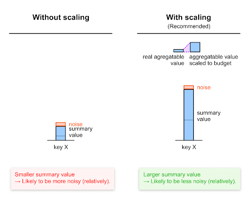
Scale up to contribution budget
As explained in Understanding noise, noise applied to the summary value for each key is based on the 0-65,536 scale (0-CONTRIBUTION_BUDGET).

Due to this, to maximize signal relative to noise, you should scale up each value before setting it as an aggregatable value—that is, multiply each value by a certain factor, the scaling factor, while ensuring it stays within the contribution budget.
Calculating a scaling factor
The scaling factor represents how much you want to scale a given aggregatable value. Its value should be the contribution budget divided by the maximum aggregatable value for a certain key.
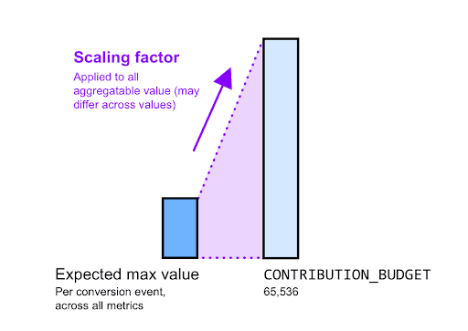
For example, let's assume advertisers want to know the total purchase value. You know that the maximum expected purchase value of any individual purchase is $2,000, except for a few outliers that you decide to ignore:
- Calculate the scaling factor:
- To maximize the signal-to-noise ratio, you need to scale this value to 65,536 (the contribution budget).
- This results in a 65,536 / 2,000 an approximately 32x scaling factor. In practice, you may round this factor up or down.
- Scale up your values before aggregation. For every $1 of purchase, increment the tracked metric by 32. For example, for a purchase of $120, set an aggregatable value of 120*32 = 3,840.
- Scale down your values after aggregation. Once you receive the summary report that contains the purchase value summed across multiple users, scale down the summary value using the scaling factor you used before aggregation. In our example, we've used a scaling factor of 32 pre-aggregation, so we need to divide the summary value received in the summary report by 32. Therefore, if the summary purchase value for a given key in the summary report is 76,800, the summary purchase value (with noise) is 76,800/32 = $2,400.
Split up your budget
If you have several measurement goals—for example, purchase count and purchase value—you may want to split your budget across these goals.
In this case, your scaling factors will be different for different aggregatable values, depending on the expected maximum of a given aggregatable value.
Read details in the Understanding aggregation keys.
For example, let's assume you're tracking both the purchase count and the purchase value, and that you decide to allocate your budget equally.
65,536 / 2 = 32,768 can be allocated per measurement type and per source.
- Purchase count:
- You're only tracking one purchase, so the maximum number of purchases for a given conversion is 1.
- Therefore, you decide to set your scaling factor for purchase count to 32,768 / 1 = 32,768.
- Purchase value:
- Let's assume the maximum expected purchase value of any individual purchase is $2,000.
- Therefore, you decide to set your scaling factor for purchase value to 32,768 / 2,000 = 16.384 or approximately 16.
Coarser aggregation keys improve signal-to-noise ratio
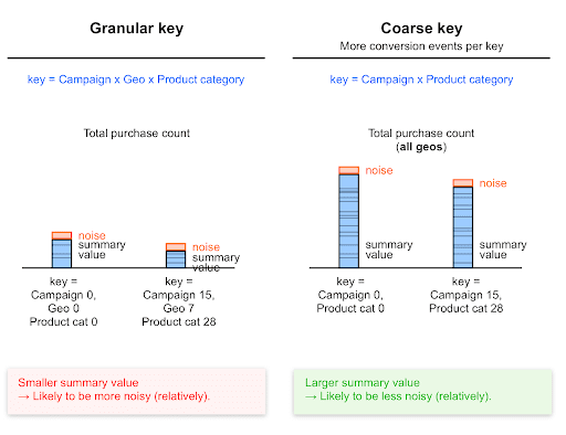
Since coarse keys catch more conversion events than granular keys, coarse keys generally lead to higher summary values.
Higher summary values are less impacted by noise than lower values; noise on these values is likely to be lower, relative to this value.
Values collected with coarser keys are likely to be relatively less noisy than values collected with more granular keys.
Example
All else held equal, a key that tracks purchase value globally (summed across all countries) will lead to a higher summary purchase value (and a higher summary conversion count) than a key that tracks conversions at a country's level.
Therefore, the relative noise on the total purchase value for a specific country will be higher than the relative noise on the total purchase value for all countries.
Similarly, all else held equal, the total purchase value for shoes is lower than the total purchase value for all items (including shoes).
Therefore, the relative noise on the total purchase value for shoes will be higher than the relative noise on the total purchase value for all items.
Summing up summary values (rollups) also sums their noise
By summing up your summary values from summary reports to access higher-level data, you also sum the noise from these summary values.
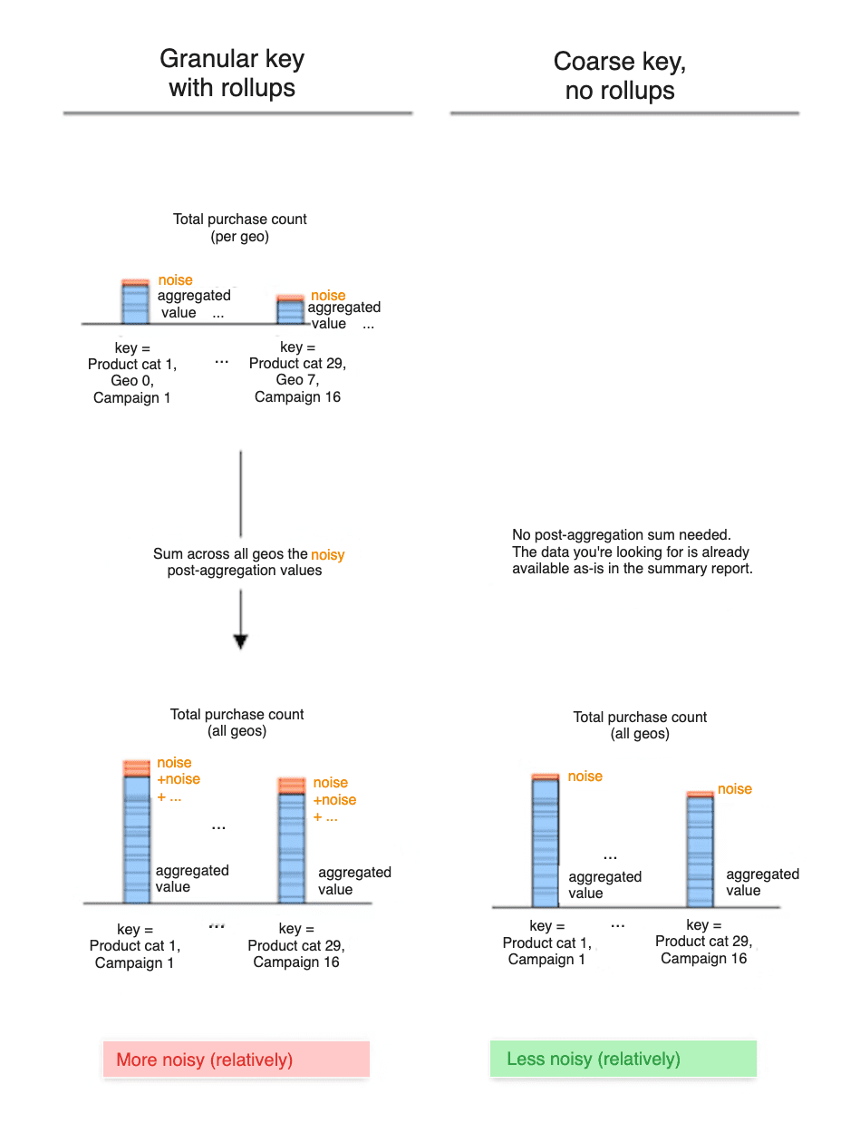
Let's look at two different approaches: - Approach A: you include a Geography ID in your keys. Summary reports expose geo-ID-level keys, each associated with the summary purchase value at a specific Geo ID's level. - Approach B: you don't include geography ID in your keys. Summary reports directly expose the summary purchase value for all geography IDs / locations.
To access country-level purchase value: - With approach A, you sum geo-ID-level summary values and hence also sum their noise. This is likely to cause more noise added to the final geo-ID-level purchase value. - With approach B, you directly look at the data exposed in summary reports. Noise has been added only once to that data.
Therefore, the summary purchase value for a given geo ID is likely to be more noisy with approach A.
Similarly, including a zipcode-level dimension in your keys will likely lead to more noisy results than using coarser keys with a region-level dimension.
Aggregating over longer time periods increases signal-to-noise ratio
Requesting summary reports less often means that each summary value will likely be higher than if you requested reports more often; more conversions are likely to happen in longer time spans.
As mentioned earlier, the higher the summary value is, the lower the relative noise is likely to be. Therefore, requesting summary reports less frequently leads to a higher (better) signal to noise ratio.
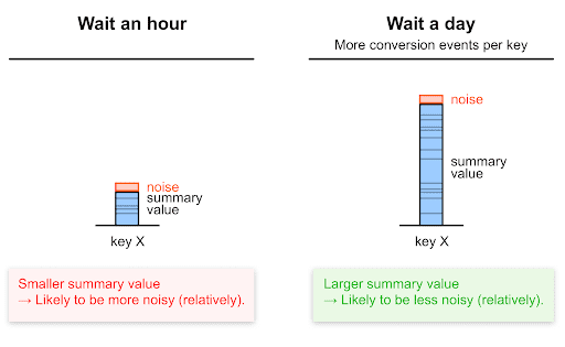
Here's an example to illustrate:
- If you're requesting hourly summary reports over 24 hours and then summing the summary value from each hourly report to access day-level data, noise is added 24 times.
- In one daily summary report, noise is added in only once.
Higher epsilon, lower noise
The higher the epsilon value, the lower the noise and the lower the privacy protection.
Leveraging filtering and deduplication
An important part of allocating budget between different keys is understanding how many times a given event can occur. For example, an advertiser may only care about one purchase for each click, but might be interested in up to 3 "product page view" conversions. To support these use-cases, you may also want to leverage the following API features that enable you to control how many reports are generated, and which conversions are counted:
- Filtering. Read more about filtering.
- Deduplication. Read more about deduplication.
Experimenting with epsilon
Ad techs can set epsilon to a value greater than 0 and up to and including 64. This range allows for flexible testing. Lower values of epsilon provide greater privacy protection. We recommend you start with epsilon=10.
Recommendations to experiment
We recommend the following: - Start with epsilon = 10. - In case this causes notable utility issues, increase epsilon incrementally. - Share your feedback about specific inflection points you may find with regards to data usability.
Engage and share feedback
You can participate and experiment with this API.
- Read about aggregatable reports and the aggregation service, ask questions, and suggest feedback.
- Read the Attribution reporting guides.
- Ask questions and join discussions on the Privacy Sandbox Developer Support repo.
Next steps
- For more information on factors that influence reporting, such as campaign variables, batching frequency, and dimension granularity, refer to Experiment with summary report design decisions .
- Try out the Noise lab.
